Chapter 11 Distributed R
Not like this. Not like this. Not like this.
— Cersei Lannister
In previous chapters, you learned how to perform data analysis and modeling in local Spark instances and proper Spark clusters. In Chapter 10 specifically, we examined how to make use of the additional functionality provided by the Spark and R communities at large. In most cases, the combination of Spark functionality and extensions is more than enough to perform almost any computation. However, for those cases in which functionality is lacking in Spark and their extensions, you could consider distributing R computations to worker nodes yourself.
You can run arbitrary R code in each worker node to run any computation—you can run simulations, crawl content from the web, transform data, and so on. In addition, you can also make use of any package available in CRAN and private packages available in your organization, which reduces the amount of code that you need to write to help you remain productive.
If you are already familiar with R, you might be tempted to use this approach for all Spark operations; however, this is not the recommended use of spark_apply(). Previous chapters provided more efficient techniques and tools to solve well-known problems; in contrast, spark_apply() introduces additional cognitive overhead, additional troubleshooting steps, performance trade-offs, and, in general, additional complexity you should avoid. Not to say that spark_apply() should never be used; rather, spark_apply() is reserved to support use cases for which previous tools and techniques fell short.
11.1 Overview
Chapter 1 introduced MapReduce as a technique capable of processing large-scale datasets. It also described how Apache Spark provided a superset of operations to perform MapReduce computations easily and more efficiently. Chapter 9 presented insights into how Spark works by applying custom transformations over each partition of the distributed datasets. For instance, if we multiplied each element of a distributed numeric dataset by 10, Spark would apply a mapping operation over each partition through multiple workers. A conceptual view of this process is illustrated in Figure 11.1.
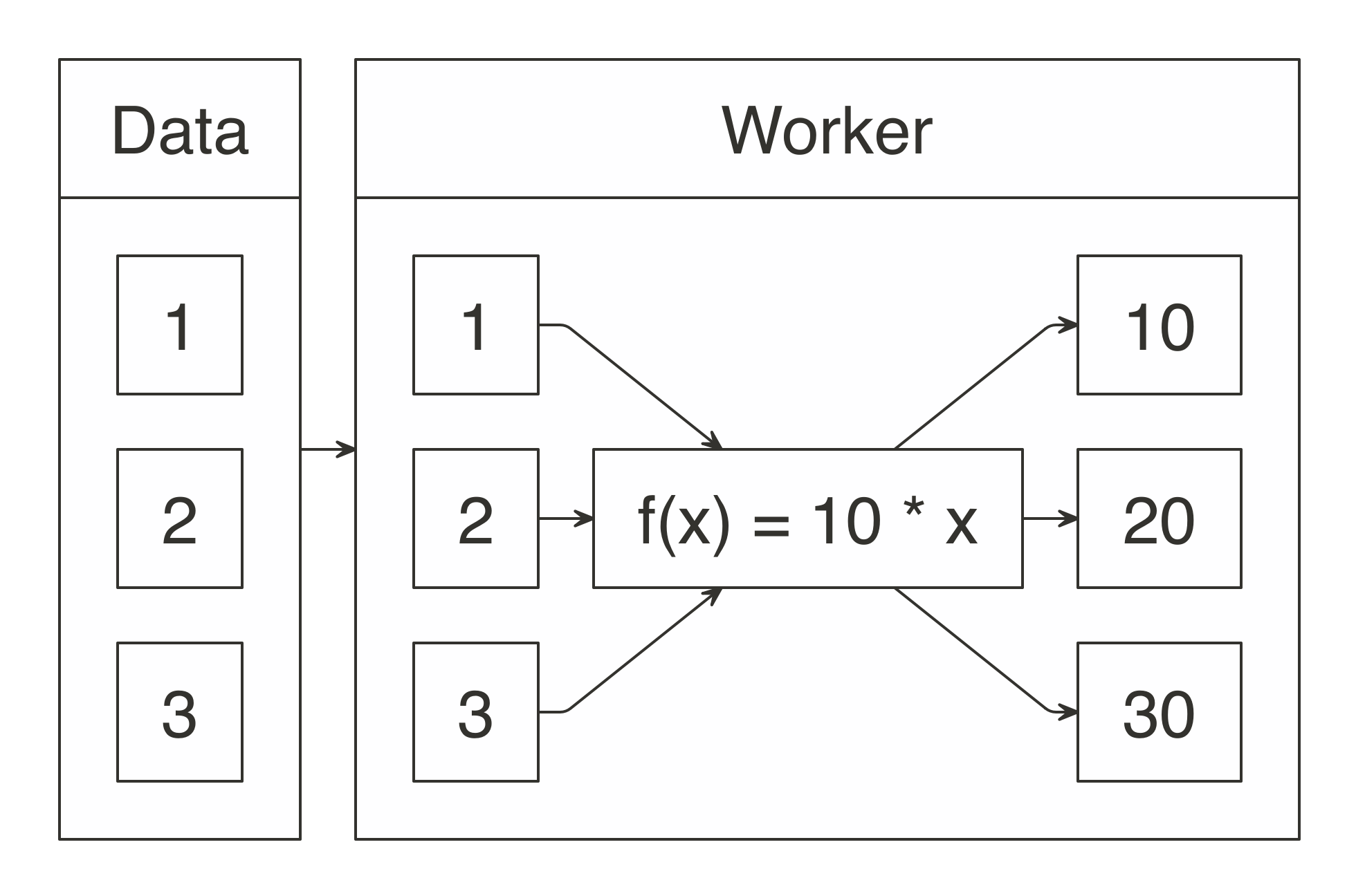
FIGURE 11.1: Map operation when multiplying by 10
This chapter presents how to define a custom f(x) mapping operation using spark_apply(); for the previous example, spark_apply() provides support to define 10 * x, as follows:
# Source: spark<?> [?? x 1]
     id
* <dbl>
1    10
2    20
3    30
Notice that ~ 10 * .x is plain R code executed across all worker nodes. The ~ operator is defined in the rlang package and provides a compact definition of a function equivalent to function(.x) 10 * .x; this compact form is also known as an anonymous function, or lambda expression.
The f(x) function must take an R DataFrame (or something that can be automatically transformed to one) as input and must also produce an R DataFrame as output, as shown in Figure 11.2.

FIGURE 11.2: Expected function signature in spark_apply() mappings
We can refer back to the original MapReduce example from Chapter 1, where the map operation was defined to split sentences into words and the total unique words were counted as the reduce operation.
In R, we could make use of the unnest_tokens() function from the tidytext R package, which you would need to install from CRAN before connecting to Spark. You can then use tidytext with spark_apply() to tokenize those sentences into a table of words:
sentences <- copy_to(sc, data_frame(text = c("I like apples", "I like bananas")))

sentences %>%
  spark_apply(~tidytext::unnest_tokens(.x, word, text))
# Source: spark<?> [?? x 1]
word
* <chr>
1 i
2 like
3 apples
4 i
5 like
6 bananasWe can complete this MapReduce example by performing the reduce operation with dplyr, as follows:
sentences %>%
  spark_apply(~tidytext::unnest_tokens(., word, text)) %>%
  group_by(word) %>%
  summarise(count = count())
# Source: spark<?> [?? x 2]
word count
* <chr> <dbl>
1 i 2
2 apples 1
3 like 2
4 bananas 1The rest of this chapter will explain in detail the use cases, features, caveats, considerations, and troubleshooting techniques required when you are defining custom mappings through spark_apply().
Note: The previous sentence tokenizer example can be more efficiently implemented using concepts from previous chapters, specifically through sentences %>% ft_tokenizer("text", "words") %>% transmute(word = explode(words)).
11.2 Use Cases
Now that we’ve presented an example to help you understand how spark_apply() works, we’ll cover a few practical use cases for it:
- Import
- You can consider using R to import data from external data sources and formats. For example, when a file format is not natively supported in Spark or its extensions, you can consider using R code to implement a distributed custom parser using R packages.
- Model
- It is natural to use the rich modeling capabilities already available in R with Spark. In most cases, R models can’t be used across large data; however, we will present two particular use cases where R models can be useful at scale. For instance, when data fits into a single machine, you can use grid search to optimize their parameters in parallel. In cases where the data can be partitioned to create several models over subsets of the data, you can use partitioned modeling in R to compute models across partitions.
- Transform
- You can use R’s rich data transformation capabilities to complement Spark. We’ll present a use case of evaluating data by external systems, and use R to interoperate with them by calling them through(((“web APIs”))) a web API.
- Compute
- When you need to perform large-scale computation in R, or big compute as described in Chapter 1, Spark is ideal to distribute this computation. We will present simulations as a particular use case for large-scale computing in R.
As we now explore each use case in detail, we’ll provide a working example to help you understand how to use spark_apply() effectively.
11.2.1 Custom Parsers
Though Spark and its various extensions provide support for many file formats (CSVs, JSON, Parquet, AVRO, etc.), you might need other formats to use at scale. You can parse these additional formats using spark_apply() and many existing R packages. In this section, we will look at how to parse logfiles, though similar approaches can be followed to parse other file formats.
It is common to use Spark to analyze logfiles—for instance, logs that track download data from Amazon S3. The webreadr package can simplify the process of parsing logs by providing support to load logs stored as Amazon S3, Squid, and the Common log format. You should install webreadr from CRAN before connecting to Spark.
For example, an Amazon S3 log looks as follows:
#Version: 1.0
#Fields: date time x-edge-location sc-bytes c-ip cs-method cs(Host) cs-uri-stem
  sc-status cs(Referer) cs(User-Agent) cs-uri-query cs(Cookie) x-edge-result-type
  x-edge-request-id x-host-header cs-protocol cs-bytes time-taken

2014-05-23  01:13:11    FRA2    182 192.0.2.10  GET d111111abcdef8.cloudfront.net
  /view/my/file.html    200 www.displaymyfiles.com  Mozilla/4.0%20
  (compatible;%20MSIE%205.0b1;%20Mac_PowerPC)   -   zip=98101   RefreshHit
  MRVMF7KydIvxMWfJIglgwHQwZsbG2IhRJ07sn9AkKUFSHS9EXAMPLE==
  d111111abcdef8.cloudfront.net http    -   0.001
This can be parsed easily with read_aws(), as follows:
# A tibble: 2 x 18
  date                edge_location bytes_sent ip_address http_method host  path
  <dttm>              <chr>              <int> <chr>      <chr>       <chr> <chr>
1 2014-05-23 01:13:11 FRA2                 182 192.0.2.10 GET         d111… /vie…
2 2014-05-23 01:13:12 LAX1             2390282 192.0.2.2… GET         d111… /sou…
# ... with 11 more variables: status_code <int>, referer <chr>, user_agent <chr>,
#   query <chr>, cookie <chr>, result_type <chr>, request_id <chr>,
#   host_header <chr>, protocol <chr>, bytes_received <chr>, time_elapsed <dbl>
To scale this operation, we can make use of read_aws() using spark_apply():
spark_read_text(sc, "logs", aws_log, overwrite = TRUE, whole = TRUE) %>%
  spark_apply(~webreadr::read_aws(.x$contents))
# Source: spark<?> [?? x 18]
date edge_location bytes_sent ip_address http_method host path
* <dttm> <chr> <int> <chr> <chr> <chr> <chr>
1 2014-05-23 01:13:11 FRA2 182 192.0.2.10 GET d111… /vie…
2 2014-05-23 01:13:12 LAX1 2390282 192.0.2.2… GET d111… /sou…
# ... with 11 more variables: status_code <int>, referer <chr>, user_agent <chr>,
# query <chr>, cookie <chr>, result_type <chr>, request_id <chr>,
# host_header <chr>, protocol <chr>, bytes_received <chr>, time_elapsed <dbl>The code used by plain R and spark_apply() is similar; however, with spark_apply(), logs are parsed in parallel across all the worker nodes available in your cluster.
This concludes the custom parsers discussion; you can parse many other file formats at scale from R following a similar approach. Next we’ll look at present partitioned modeling as another use case focused on modeling across several datasets in parallel.
11.2.2 Partitioned Modeling
There are many modeling packages available in R that can also be run at scale by partitioning the data into manageable groups that fit in the resources of a single machine.
For instance, suppose that you have a 1 TB dataset for sales data across multiple cities and you are tasked with creating sales predictions over each city. For this case, you can consider partitioning the original dataset per city—say, into 10 GB of data per city—which could be managed by a single compute instance. For this kind of partitionable dataset, you can also consider using spark_apply() by training each model over each city.
As a simple example of partitioned modeling, we can run a linear regression using the iris dataset partitioned by species:
# Source: spark<?> [?? x 2]
  Species    result
  <chr>       <int>
1 versicolor     50
2 virginica      50
3 setosa         50
Then you can run a linear regression over each species using spark_apply():
iris %>%
  spark_apply(
    function(e) summary(lm(Petal_Length ~ Petal_Width, e))$r.squared,
    names = "r.squared",
    group_by = "Species")
# Source: spark<?> [?? x 2]
Species r.squared
<chr> <dbl>
1 versicolor 0.619
2 virginica 0.104
3 setosa 0.110As you can see from the r.squared results and intuitively in Figure 11.3, the linear model for versicolor better fits to the regression line:
purrr::map(c("versicolor", "virginica", "setosa"),
  ~dplyr::filter(datasets::iris, Species == !!.x) %>%
    ggplot2::ggplot(ggplot2::aes(x = Petal.Length, y = Petal.Width)) +
    ggplot2::geom_point())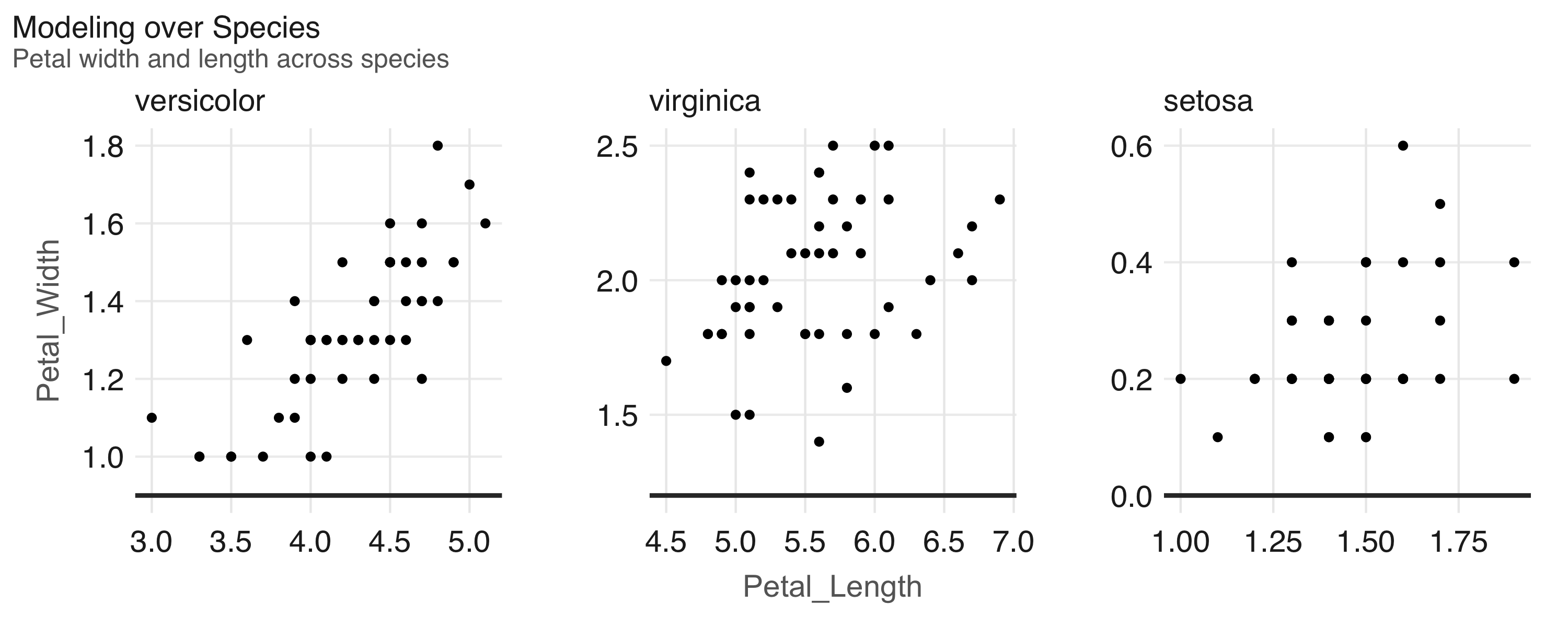
FIGURE 11.3: Modeling over species in the iris dataset
This concludes our brief overview on how to perform modeling over several different partitionable datasets. A similar technique can be applied to perform modeling over the same dataset using different modeling parameters, as we cover next.
11.2.3 Grid Search
Many R packages provide models that require defining multiple parameters to configure and optimize. When the value of these parameters is unknown, we can distribute this list of unknown parameters across a cluster of machines to find the optimal parameter combination. If the list contains more than one parameter to optimize, it is common to test against all the combinations between parameter A and parameter B, creating a grid of parameters. The process of searching for the best parameter over this parameter grid is commonly known as grid search.
For example, we can define a grid of parameters to optimize decision tree models as follows:
grid <- list(minsplit = c(2, 5, 10), maxdepth = c(1, 3, 8)) %>%
  purrr:::cross_df() %>%
  copy_to(sc, ., repartition = 9)
grid
# Source: spark<?> [?? x 2]
minsplit maxdepth
<dbl> <dbl>
1 2 1
2 5 1
3 10 1
4 2 3
5 5 3
6 10 3
7 2 8
8 5 8
9 10 8The grid dataset was copied by using repartition = 9 to ensure that each partition is contained in one machine, since the grid also has nine rows. Now, assuming that the original dataset fits in every machine, we can distribute this dataset to many machines and perform parameter search to find the model that best fits this data:
spark_apply(
  grid,
  function(grid, cars) {
    model <- rpart::rpart(
      am ~ hp + mpg,
      data = cars,
      control = rpart::rpart.control(minsplit = grid$minsplit,
                                     maxdepth = grid$maxdepth)
    )
    dplyr::mutate(
      grid,
      accuracy = mean(round(predict(model, dplyr::select(cars, -am))) == cars$am)
    )
  },
  context = mtcars)
# Source: spark<?> [?? x 3]
minsplit maxdepth accuracy
<dbl> <dbl> <dbl>
1 2 1 0.812
2 5 1 0.812
3 10 1 0.812
4 2 3 0.938
5 5 3 0.938
6 10 3 0.812
7 2 8 1
8 5 8 0.938
9 10 8 0.812For this model, minsplit = 2 and maxdepth = 8 produces the most accurate results. You can now use this specific parameter combination to properly train your model.
11.2.4 Web APIs
A web API is a program that can do something useful through a web interface that other programs can reuse. For instance, services like Twitter provide web APIs that allow you to automate reading tweets from a program written in R and other programming languages. You can make use of web APIs using spark_apply() by sending programmatic requests to external services using R code.
For example, Google provides a web API to label images using deep learning techniques; you can use this API from R, but for larger datasets, you need to access its APIs from Spark. You can use Spark to prepare data to be consumed by a web API and then use spark_apply() to perform this call and process all the incoming results back in Spark.
The next example makes use of the googleAuthR package to authenticate to Google Cloud, the RoogleVision package to perform labeling over the Google Vision API, and spark_apply() to interoperate between Spark and Google’s deep learning service. To run the following example, you’ll first need to disconnect from Spark and download your cloudml.json file from the Google developer portal:
sc <- spark_connect(
  master = "local",
  config = list(sparklyr.shell.files = "cloudml.json"))

images <- copy_to(sc, data.frame(
  image = "http://pbs.twimg.com/media/DwzcM88XgAINkg-.jpg"
))

spark_apply(images, function(df) {
  googleAuthR::gar_auth_service(
    scope = "https://www.googleapis.com/auth/cloud-platform",
    json_file = "cloudml.json")

  RoogleVision::getGoogleVisionResponse(
    df$image,
    download = FALSE)
})
# Source: spark<?> [?? x 4]
mid description score topicality
<chr> <chr> <dbl> <dbl>
1 /m/04rky Mammal 0.973 0.973
2 /m/0bt9lr Dog 0.958 0.958
3 /m/01z5f Canidae 0.956 0.956
4 /m/0kpmf Dog breed 0.909 0.909
5 /m/05mqq3 Snout 0.891 0.891To successfully run a large distributed computation over a web API, the API needs to be able to scale to support the load from all the Spark executors. We can trust that major service providers are likely to support all the requests incoming from your cluster. But when you’re calling internal web APIs, make sure the API can handle the load. Also, when you’re using third-party services, consider the cost of calling their APIs across all the executors in your cluster to avoid potentially expensive and unexpected charges.
Next we’ll describe a use case for big compute where R is used to perform distributed rendering.
11.2.5 Simulations
You can use R combined with Spark to perform large-scale computing. The use case we explore here is rendering computationally expensive images using the rayrender package, which uses ray tracing, a photorealistic technique commonly used in movie production.
Let’s use this package to render a simple scene that includes a few spheres (see Figure 11.4) that use a lambertian material, a diffusely reflecting material or “matte”. First, install rayrender using install.packages("rayrender"). Then, be sure you’ve disconnected and reconnected Spark:
library(rayrender)

scene <- generate_ground(material = lambertian()) %>%
  add_object(sphere(material = metal(color="orange"), z = -2)) %>%
  add_object(sphere(material = metal(color="orange"), z = +2)) %>%
  add_object(sphere(material = metal(color="orange"), x = -2))

render_scene(scene, lookfrom = c(10, 5, 0), parallel = TRUE)
FIGURE 11.4: Ray tracing in Spark using R and rayrender
In higher resolutions, say 1920 x 1080, the previous example takes several minutes to render the single frame from Figure 11.4; rendering a few seconds at 30 frames per second would take several hours in a single machine. However, we can reduce this time using multiple machines by parallelizing computation across them. For instance, using 10 machines with the same number of CPUs would cut rendering time tenfold:
system2("hadoop", args = c("fs", "-mkdir", "/rendering"))

sdf_len(sc, 628, repartition = 628) %>%
  spark_apply(function(idx, scene) {
    render <- sprintf("%04d.png", idx$id)
    rayrender::render_scene(scene, width = 1920, height = 1080,
                            lookfrom = c(12 * sin(idx$id/100),
                                         5, 12 * cos(idx$id/100)),
                            filename = render)

    system2("hadoop", args = c("fs", "-put", render, "/user/hadoop/rendering/"))
  }, context = scene, columns = list()) %>% collect()
After all the images are rendered, the last step is to collect them from HDFS and use tools like ffmpeg to convert individual images into an animation:
hadoop fs -get rendering/
ffmpeg -s 1920x1080 -i rendering/%d.png -vcodec libx264 -crf 25
       -pix_fmt yuv420p rendering.mp4
Note: This example assumes HDFS is used as the storage technology for Spark and being run under a hadoop user, you will need to adjust this for your particular storage or user.
We’ve covered some common use cases for spark_apply(), but you are certainly welcome to find other use cases for your particular needs. The next sections present technical concepts you’ll need to understand to create additional use cases and to use spark_apply() effectively.
11.3 Partitions
Most Spark operations that analyze data with dplyr or model with MLlib don’t require understanding how Spark partitions data; they simply work automatically. However, for distributed R computations, this is not the case. For these you will have to learn and understand how exactly Spark is partitioning your data and provide transformations that are compatible with them. This is required since spark_apply() receives each partition and allows you to perform any transformation, not the entire dataset. You can refresh concepts like partitioning and transformations using the diagrams and examples from Chapter 9.
To help you understand how partitions are represented in spark_apply(), consider the following code:
# Source: spark<?> [?? x 1]
  result
*  <int>
1      5
2      5
Should we expect the output to be the total number of rows? As you can see from the results, in general the answer is no; Spark assumes data will be distributed across multiple machines, so you’ll often find it already partitioned, even for small datasets. Because we should not expect spark_apply() to operate over a single partition, let’s find out how many partitions sdf_len(sc, 10) contains:
[1] 2This explains why counting rows through nrow() under spark_apply() retrieves two rows since there are two partitions, not one. spark_apply() is retrieving the count of rows over each partition, and each partition contains 5 rows, not 10 rows total, as you might have expected.
For this particular example, we could further aggregate these partitions by repartitioning and then adding up—this would resemble a simple MapReduce operation using spark_apply():
# Source: spark<?> [?? x 1]
  result
*  <int>
1     10
So now that you know about partitions using spark_apply(), we’ll move on to using group_by to control partitions.
11.4 Grouping
When using spark_apply(), we can request explicit partitions from Spark. For instance, if we had to process numbers less than four in one partition and the remaining ones in a second partition, we could create these groups explicitly and then request spark_apply() to use them:
# Source: spark<?> [?? x 2]
  groups result
* <lgl>   <int>
1 TRUE        3
2 FALSE       7
Notice that spark_apply() is still processing two partitions, but in this case we expect these partitions since we explicitly requested them in spark_apply(); therefore, you can safely interpret the results as “there are three integers less than four”.
Note: You can only group data by partitions that fit in a single machine; if one of the groups is too large, an exception will be thrown. To perform operations over groups that exceed the resources of a single node, you can consider partitioning to smaller units or use dplyr::do, which is currently optimized for large partitions.
The takeaway from this section is to always consider partitions when dealing with spark_apply(). Next, we will zoom in to spark_apply() to understand how columns are interpreted.
11.5 Columns
By default, spark_apply() automatically inspects the DataFrame being produced to learn column names and types. For example:
# Source: spark<?> [?? x 2]
  numbers names
*   <dbl> <chr>
1       1 abc
However, this is inefficient since spark_apply() needs to run twice: first, to find columns by computing spark_apply() against a subset of all the data, and then to compute the actual desired values.
To improve performance, you can explicitly specify the columns through the columns parameters. This parameter takes a named list of types expected in the resulting DataFrame. We can then rewrite the previous example to run only once by specifying the correct type for the numbers column:
sdf_len(sc, 1) %>%
  spark_apply(
    ~ data.frame(numbers = 1, names = "abc"),
    columns = list(numbers = "double", names = "character"))
# Source: spark<?> [?? x 2]
numbers names
* <dbl> <chr>
1 1 abc Now that we’ve presented how rows and columns interact with spark_apply(), let’s move on to making use of the contextual information sometimes required when processing distributed datasets.
11.6 Context
To process partitions using spark_apply(), you might need to include auxiliary data that is small enough to fit in each node. This was the case in the grid search use case, where the dataset was passed to all partitions and remained unpartitioned itself.
We can modify the initial f(x) = 10 * x example in this chapter to customize the multiplier. It was originally set to 10, but we can make it configurable by specifying it as the context parameter:
# Source: spark<?> [?? x 1]
     id
  <dbl>
1   100
2   200
3   300
4   400
Figure 11.5 illustrates this example conceptually. Notice that the data partitions are still variable; however, the contextual parameter is distributed to all the nodes.
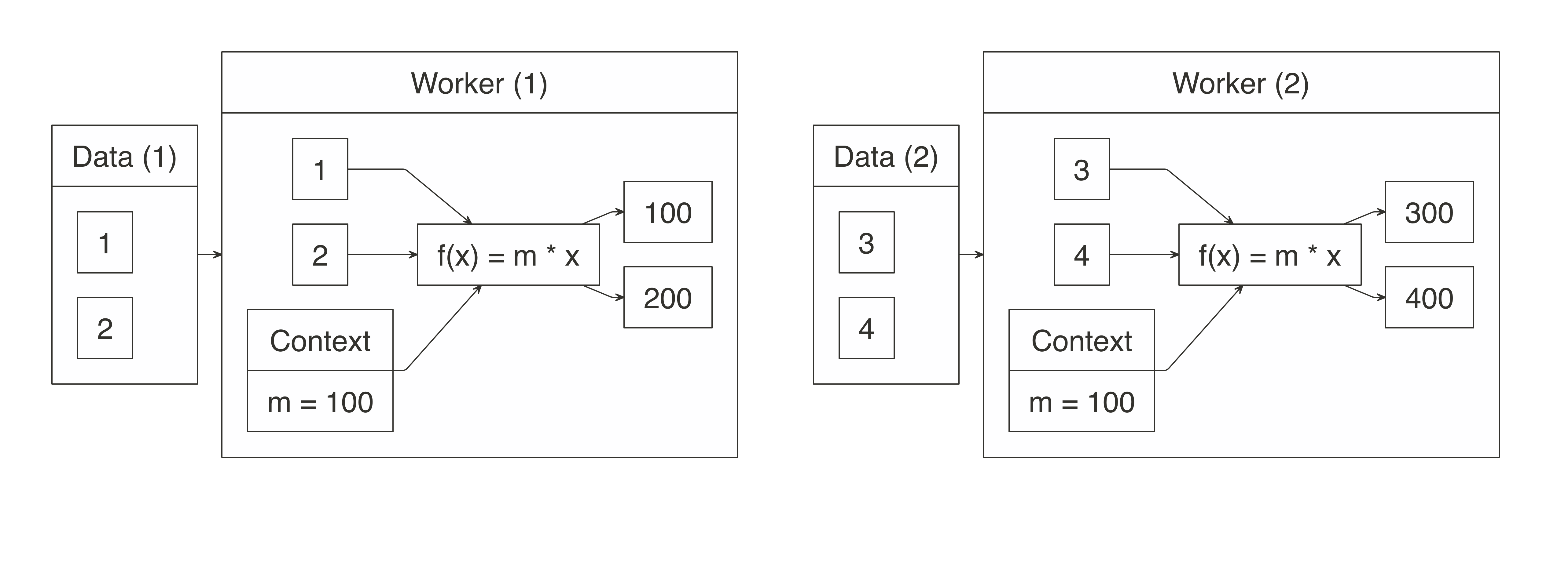
FIGURE 11.5: Map operation when multiplying with context
The grid search example used this parameter to pass a DataFrame to each worker node; however, since the context parameter is serialized as an R object, it can contain anything. For instance, if you need to pass multiple values—or even multiple datasets—you can pass a list with values.
The following example defines a f(x) = m * x + b function and runs m = 10 and b = 2:
# Source: spark<?> [?? x 1]
     id
  <dbl>
1    12
2    22
3    32
4    42
Notice that we’ve renamed context to .y to shorten the variable name. This works because spark_apply() assumes context is the second parameter in functions and expressions.
You’ll find the context parameter extremely useful; for instance, the next section presents how to properly construct functions, and context is used in advanced use cases to construct functions dependent on other functions.
11.7 Functions
Earlier we presented spark_apply() as an operation to perform custom transformations using a function or expression. In programming literature, functions with a context are also referred to as a closure.
Expressions are useful to define short transformations, like ~ 10 * .x. For an expression, .x contains a partition and .y the context, when available. However, it can be hard to define an expression for complex code that spans multiple lines. For those cases, functions are more appropriate.
Functions enable complex and multiline transformations, and are defined as function(data, context) {} where you can provide arbitrary code within the {}. We’ve seen them in previous sections when using Google Cloud to transform images into image captions.
The function passed to spark_apply() is serialized using serialize(), which is described as “a simple low-level interface for serializing to connections”. One current limitation of serialize() is that it won’t serialize objects being referenced outside its environment. For instance, the following function errors out since the closure references external_value:
As workarounds to this limitation, you can add the functions your closure needs into the context and then assign the functions into the global environment:
func_a <- function() 40
func_b <- function() func_a() + 1
func_c <- function() func_b() + 1

sdf_len(sc, 1) %>% spark_apply(function(df, context) {
  for (name in names(context)) assign(name, context[[name]], envir = .GlobalEnv)
  func_c()
}, context = list(
  func_a = func_a,
  func_b = func_b,
  func_c = func_c
))
# Source: spark<?> [?? x 1]
result
<dbl>
1 42When this isn’t feasible, you can also create your own R package with the functionality you need and then use your package in spark_apply().
You’ve learned all the functionality available in spark_apply() using plain R code. In the next section we present how to use packages when distributing computations. R packages are essential when you are creating useful transformations.
11.8 Packages
With spark_apply() you can use any R package inside Spark. For instance, you can use the broom package to create a tidy(((“DataFrames”, “from linear regression output”))) DataFrame from linear regression output:
spark_apply(
  iris,
  function(e) broom::tidy(lm(Petal_Length ~ Petal_Width, e)),
  names = c("term", "estimate", "std.error", "statistic", "p.value"),
  group_by = "Species")
# Source: spark<?> [?? x 6]
Species term estimate std.error statistic p.value
<chr> <chr> <dbl> <dbl> <dbl> <dbl>
1 versicolor (Intercept) 1.78 0.284 6.28 9.48e- 8
2 versicolor Petal_Width 1.87 0.212 8.83 1.27e-11
3 virginica (Intercept) 4.24 0.561 7.56 1.04e- 9
4 virginica Petal_Width 0.647 0.275 2.36 2.25e- 2
5 setosa (Intercept) 1.33 0.0600 22.1 7.68e-27
6 setosa Petal_Width 0.546 0.224 2.44 1.86e- 2The first time you call spark_apply(), all the contents in your local .libPaths() (which contains all R packages) will be copied into each Spark worker node. Packages are only copied once and persist as long as the connection remains open. It’s not uncommon for R libraries to be several gigabytes in size, so be prepared for a one-time tax while the R packages are copied over to your Spark cluster. You can disable package distribution by setting packages = FALSE.
Note: Since packages are copied only once for the duration of the spark_connect() connection, installing additional packages is not supported while the connection is active. Therefore, if a new package needs to be installed, spark_disconnect() the connection, modify packages, and then reconnect. In addition, R packages are not copied in local mode, because the packages already exist on the local system.
Though this section was brief, using packages with distributed R code opens up an entire new universe of interesting use cases. Some of those use cases were presented in this chapter, but by looking at the rich ecosystem of R packages available today you’ll find many more.
This section completes our discussion of the functionality needed to distribute R code with R packages. We’ll now cover some of the requirements your cluster needs to make use of spark_apply().
11.9 Cluster Requirements
The functionality presented in previous chapters did not require special configuration of your Spark cluster—as long as you had a properly configured Spark cluster, you could use R with it. However, for the functionality presented here, your cluster administrator, cloud provider, or you will have to configure your cluster by installing either:
- R in every node, to execute R code across your cluster
- Apache Arrow in every node when using Spark 2.3 or later (Arrow provides performance improvements that bring distributed R code closer to native Scala code)
Let’s take a look at each requirement to ensure that you properly consider the trade-offs or benefits that they provide.
11.9.1 Installing R
Starting with the first requirement, the R runtime is expected to be preinstalled in every node in the cluster; this is a requirement specific to spark_apply().
Failure to install R in every node will trigger a Cannot run program, no such file or directory error when you attempt to use spark_apply().
Contact your cluster administrator to consider making the R runtime available throughout the entire cluster. If R is already installed, you can specify the installation path to use with the spark.r.command configuration setting, as shown here:
config <- spark_config()
config["spark.r.command"] <- "<path-to-r-version>"

sc <- spark_connect(master = "local", config = config)
sdf_len(sc, 10) %>% spark_apply(function(e) e)
A homogeneous cluster is required since the driver node distributes, and potentially compiles, packages to the workers. For instance, the driver and workers must have the same processor architecture, system libraries, and so on. This is usually the case for most clusters, but might not be true for yours.
Different cluster managers, Spark distributions, and cloud providers support different solutions to install additional software (like R) across every node in the cluster; follow instructions when installing R over each worker node. Here are a few examples:
- Spark Standalone
- Requires connecting to each machine and installing R; tools like
psshallow you to run a single installation command against multiple machines. - Cloudera
- Provides an R parcel (see the Cloudera blog post “How to Distribute Your R code with sparklyr and Cloudera Data Science Workbench”), which enables R over each worker node.
- Amazon EMR
- R is preinstalled when starting an EMR cluster as mentioned in Clusters - Amazon EMR.
- Microsoft HDInsight
- R is preinstalled and no additional steps are needed.
- Livy
- Livy connections do not support distributing packages because the client machine where the libraries are precompiled might not have the same processor architecture or operating systems as the cluster machines.
Strictly speaking, this completes the last requirement for your cluster. However, we strongly recommend you use Apache Arrow with spark_apply() to support large-scale computation with minimal overhead.
11.9.2 Apache Arrow
Before introducing Apache Arrow, we’ll discuss how data is stored and transferred between Spark and R. As R was designed from its inception to perform fast numeric computations to accomplish this, it’s important to figure out the best way to store data.
Some computing systems store data internally by row; however, most interesting numerical operations require data to be processed by column. For example, calculating the mean of a column requires processing each column on its own, not the entire row. Spark stores data by default by row, since it’s easier to partition; in contrast, R stores data by column. Therefore, something needs to transform both representations when data is transferred between Spark and R, as shown in Figure 11.6.
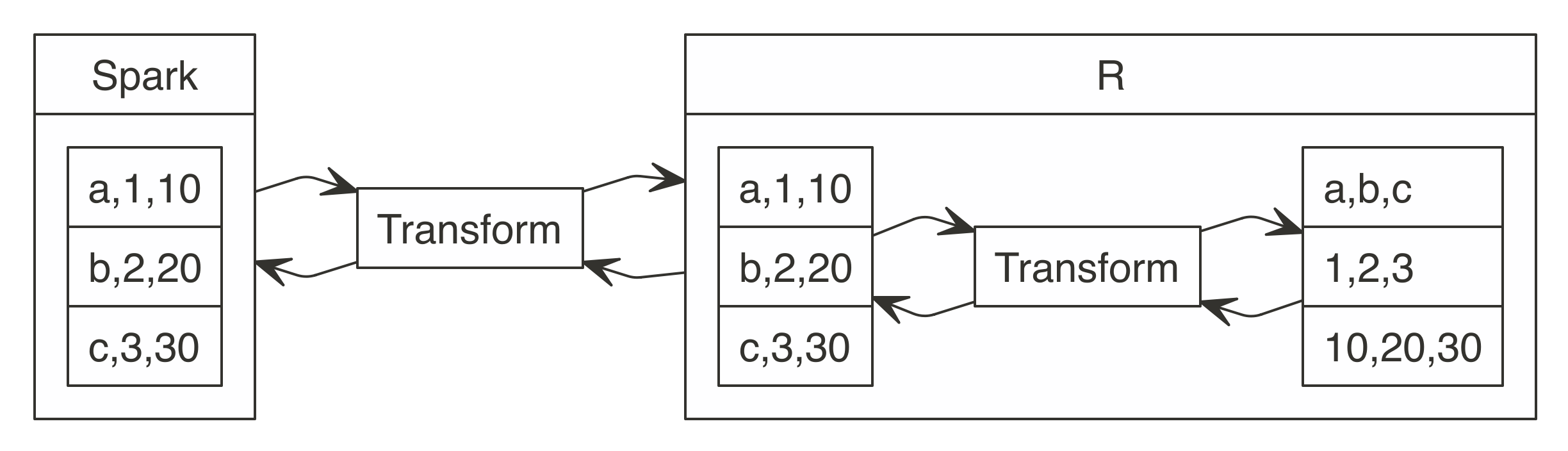
FIGURE 11.6: Data transformation between Spark and R
This transformation from rows to columns needs to happen for each partition. In addition, data also must be transformed from Scala’s internal representation to R’s internal representation. Apache Arrow reduces these transformations that waste a lot of CPU cycles.
Apache Arrow is a cross-language development platform for in-memory data. In Spark, it speeds up transferring data between Scala and R by defining a common data format compatible with many programming languages. Instead of having to transform between Scala’s internal representation and R’s, you can use the same structure for both languages. In addition, transforming data from row-based storage to columnar storage is performed in parallel in Spark, which can be further optimized by using the columnar storage formats presented in Chapter 8. The improved transformations are shown in Figure 11.6.
FIGURE 11.7: Data transformation between Spark and R using Apache Arrow
Apache Arrow is not required but is strongly recommended while you are working with spark_apply(). It has been available since Spark 2.3.0; however, it requires system administrators to install the Apache Arrow runtime in every node (see http://arrow.apache.org/install/).
In addition, to use Apache Arrow with sparklyr, you also need to install the arrow package:
Before we use arrow, let’s take a measurement to validate:
   user  system elapsed
  0.240   0.020   7.957
In our particular system, processing 10,000 rows takes about 8 seconds. To enable Arrow, simply include the library and use spark_apply() as usual. Let’s measure how long it takes spark_apply() to process 1 million rows:
   user  system elapsed
  0.317   0.021   3.922
In our system, Apache Arrow can process 100 times more data in half the time: just 4 seconds.
Most functionality in arrow simply works in the background, improving performance and data serialization; however, there is one setting you should be aware of. The spark.sql.execution.arrow.maxRecordsPerBatch configuration setting specifies the default size of each arrow data transfer. It’s shared with other Spark components and defaults to 10,000 rows:
# Source: spark<?> [?? x 1]
  result
   <int>
1  10000
2  10000
You might need to adjust this number based on how much data your system can handle, making it smaller for large datasets or bigger for operations that require records to be processed together. We can change this setting to 5,000 rows and verify the partitions change appropriately:
config <- spark_config()
config$spark.sql.execution.arrow.maxRecordsPerBatch <- 5 * 10^3

sc <- spark_connect(master = "local", config = config)
sdf_len(sc, 2 * 10^4) %>% spark_apply(nrow)
# Source: spark<?> [?? x 1]
result
<int>
1 5000
2 5000
3 5000
4 5000So far we’ve presented use cases, main operations, and cluster requirements. Now we’ll discuss the troubleshooting techniques useful when distributing R code.
11.10 Troubleshooting
A custom transformation can fail for many reasons. To learn how to troubleshoot errors, let’s simulate a problem by triggering an error ourselves:
Error in force(code) :
  sparklyr worker rscript failure, check worker logs for details
    Log: wm_bx4cn70s6h0r5vgsldm0000gn/T/Rtmpob83LD/file2aac1a6188_spark.log

---- Output Log ----
19/03/11 14:12:24 INFO sparklyr: Worker (1) completed wait using lock for RScript
Notice that the error message mentions inspecting the logs. When running in local mode, you can simply run the following:
19/03/11 14:12:24 ERROR sparklyr: RScript (1) terminated unexpectedly:
                                              force an error
This points to the artificial stop("force an error") error we mentioned. However, if you’re not working in local mode, you will have to retrieve the worker logs from your cluster manager. Since this can be cumbersome, one alternative is to rerun spark_apply() but return the error message yourself:
# Source: spark<?> [?? x 1]
  result
  <chr>
1 force an error
Among the other, more advanced troubleshooting techniques applicable to spark_apply(), the following sections present these techniques in order. You should try to troubleshoot by using worker logs first, then identifying partitioning errors, and finally, attempting to debug a worker node.
11.10.1 Worker Logs
Whenever spark_apply() is executed, information regarding execution is written over each worker node. You can use this log to write custom messages to help you diagnose and fine-tune your code.
For instance, suppose that we don’t know what the first column name of df is. We can write a custom log message executed from the worker nodes using worker_log() as follows:
sdf_len(sc, 1) %>% spark_apply(function(df) {
  worker_log("the first column in the data frame is named ", names(df)[[1]])
  df
})
# Source: spark<?> [?? x 1]
id
* <int>
1 1When running locally, we can filter the log entries for the worker as follows:
18/12/18 11:33:47 INFO sparklyr: RScript (3513) the first column in the dataframe
                                                is named id
18/12/18 11:33:47 INFO sparklyr: RScript (3513) computed closure
18/12/18 11:33:47 INFO sparklyr: RScript (3513) updating 1 rows
18/12/18 11:33:47 INFO sparklyr: RScript (3513) updated 1 rows
18/12/18 11:33:47 INFO sparklyr: RScript (3513) finished apply
18/12/18 11:33:47 INFO sparklyr: RScript (3513) finished
Notice that the logs print our custom log entry, showing that id is the name of the first column in the given DataFrame.
This functionality is useful when troubleshooting errors; for instance, if we force an error using the stop() function:
We will get an error similar to the following:
 Error in force(code) :
  sparklyr worker rscript failure, check worker logs for details
As suggested by the error, we can look in the worker logs for the specific errors as follows:
This will show an entry containing the error and the call stack:
18/12/18 11:26:47 INFO sparklyr: RScript (1860) computing closure
18/12/18 11:26:47 ERROR sparklyr: RScript (1860) terminated unexpectedly:
                                                 force an error
18/12/18 11:26:47 ERROR sparklyr: RScript (1860) collected callstack:
11: stop("force and error")
10: (function (df)
{
    stop("force and error")
})(structure(list(id = 1L), class = "data.frame", row.names = c(NA,
-1L)))
Notice that spark_log(sc) only retrieves the worker logs when you’re using local clusters. When running in proper clusters with multiple machines, you will have to use the tools and user interface provided by the cluster manager to find these log entries.
11.10.2 Resolving Timeouts
When you are running with several hundred executors, it becomes more likely that some tasks will hang indefinitely. In this situation, most of the tasks in your job complete successfully, but a handful of them are still running and do not fail or succeed.
Suppose that you need to calculate the size of many web pages. You could use spark_apply() with something similar to:
sdf_len(sc, 3, repartition = 3) %>%
  spark_apply(~ download.file("https://google.com", "index.html") +
                file.size("index.html"))
Some web pages might not exist or take too long to download. In this case, most tasks will succeed, but a few will hang. To prevent these few tasks from blocking all computations, you can use the spark.speculation Spark setting. With this setting enabled, once 75% of all tasks succeed, Spark will look for tasks taking longer than the median task execution time and retry. You can use the spark.speculation.multiplier setting to configure the time multiplier used to determine when a task is running slow.
Therefore, for this example, you could configure Spark to retry tasks that take four times longer than the median as follows:
11.10.3 Inspecting Partitions
If a particular partition fails, you can detect the broken partition by computing a digest and then retrieving that particular partition. As usual, you can install digest from CRAN before connecting to Spark:
sdf_len(sc, 3) %>% spark_apply(function(x) {
    worker_log("processing ", digest::digest(x), " partition")
    # your code
    x
})
This will add an entry similar to:
18/11/03 14:48:32 INFO sparklyr: RScript (2566)
  processing f35b1c321df0162e3f914adfb70b5416 partition
When executing this in your cluster, look in the logs for the task that is not finishing. Once you have that digest, you can cancel the job. Then you can use that digest to retrieve the specific DataFrame to R with something like this:
sdf_len(sc, 3) %>% spark_apply(function(x) {
    if (identical(digest::digest(x),
                  "f35b1c321df0162e3f914adfb70b5416")) x else x[0,]
}) %>% collect()
# A tibble: 1 x 1
result
<int>
1 1You can then run this in R to troubleshoot further.
11.10.4 Debugging Workers
A debugger is a tool that lets you execute your code line by line; you can use this to troubleshoot spark_apply() for local connections. You can start spark_apply() in debug mode by using the debug parameter and then following the instructions:
Debugging spark_apply(), connect to worker debugging session as follows:
  1. Find the workers <sessionid> and <port> in the worker logs, from RStudio
     click 'Log' under the connection, look for the last entry with contents:
     'Session (<sessionid>) is waiting for sparklyr client to connect to
      port <port>'
  2. From a new R session run:
     debugonce(sparklyr:::spark_worker_main)
     sparklyr:::spark_worker_main(<sessionid>, <port>)
As these instructions indicate, you’ll need to connect “as the worker node” from a different R session and then step through the code. This method is less straightforward than previous ones, since you’ll also need to step through some lines of sparklyr code; thus, we only recommend this as a last resort. (You can also try the online resources described in Chapter 2.)
Let’s now wrap up this chapter with a brief recap of the functionality we presented.
11.11 Recap
This chapter presented spark_apply() as an advanced technique you can use to fill gaps in functionality in Spark or its many extensions. We presented example use cases for spark_apply() to parse data, model in parallel many small datasets, perform a grid search, and call web APIs. You learned how partitions relate to spark_apply(), and how to create custom groups, distribute contextual information across all nodes, and troubleshoot problems, limitations, and cluster configuration caveats.
We also strongly recommended using Apache Arrow as a library when working with Spark with R, and presented installation, use cases, and considerations you should be aware of.
Up to this point, we’ve only worked with large datasets of static data, which doesn’t change over time and remains invariant while we analyze, model, and visualize them. In Chapter 12, we will introduce techniques to process datasets that, in addition to being large, are also growing in such a way that they resemble a stream of information.