Chapter 9 Tuning
Chaos isn’t a pit. Chaos is a ladder.
— Petyr Baelish
In previous chapters, we’ve assumed that computation within a Spark cluster works efficiently. While this is true in some cases, it is often necessary to have some knowledge of the operations Spark runs internally to fine-tune configuration settings that will make computations run efficiently. This chapter explains how Spark computes data over large datasets and provides details on how to optimize its operations.
For instance, in this chapter you’ll learn how to request more compute nodes and increase the amount of memory, which, if you remember from Chapter 2, defaults to only 2 GB in local instances. You will learn how Spark unifies computation through partitioning, shuffling, and caching. As mentioned a few chapters back, this is the last chapter describing the internals of Spark; after you complete this chapter, we believe that you will have the intermediate Spark skills necessary to be productive at using Spark.
In Chapters 10–12 we explore exciting techniques to deal with specific modeling, scaling, and computation problems. However, we must first understand how Spark performs internal computations, what pieces we can control, and why.
9.1 Overview
Spark performs distributed computation by configuring, partitioning, executing, shuffling, caching, and serializing data, tasks, and resources across multiple machines:
- Configuring requests the cluster manager for resources: total machines, memory, and so on.
- Partitioning splits the data among various machines. Partitions can be either implicit or explicit.
- Executing means running an arbitrary transformation over each partition.
- Shuffling redistributes data to the correct machine.
- Caching preserves data in memory across different computation cycles.
- Serializing transforms data to be sent over the network to other workers or back to the driver node.
To illustrate each concept, let’s create three partitions with unordered integers and then sort them using arrange():
data <- copy_to(sc,
  data.frame(id = c(4, 9, 1, 8, 2, 3, 5, 7, 6)),
  repartition = 3)

data %>% arrange(id) %>% collect()
Figure 9.1 shows how this sorting job would conceptually work across a cluster of machines. First, Spark would configure the cluster to use three worker machines. In this example, the numbers 1 through 9 are partitioned across three storage instances. Since the data is already partitioned, each worker node loads this implicit partition; for instance, 4, 9, and 1 are loaded in the first worker node. Afterward, a task is distributed to each worker to apply a transformation to each data partition in each worker node; this task is denoted by f(x). In this example, f(x) executes a sorting operation within a partition. Since Spark is general, execution over a partition can be as simple or complex as needed.
The result is then shuffled to the correct machine to finish the sorting operation across the entire dataset, which completes a stage. A stage is a set of operations that Spark can execute without shuffling data between machines. After the data is sorted across the cluster, the sorted results can be optionally cached in memory to avoid rerunning this computation multiple times.
Finally, a small subset of the results is serialized, through the network connecting the cluster machines, back to the driver node to print a preview of this sorting example.
Notice that while Figure 9.1 describes a sorting operation, a similar approach applies to filtering or joining datasets and analyzing and modeling data at scale. Spark provides support to perform custom partitions, custom shuffling, and so on, but most of these lower-level operations are not exposed in sparklyr; instead, sparklyr makes those operations available through higher-level commands provided by data analysis tools like dplyr or DBI, modeling, and by using many extensions. For those few cases in which you might need to implement low-level operations, you can always use Spark’s Scala API through sparklyr extensions or run custom distributed R code.
To effectively tune Spark, we will start by getting familiar with Spark’s computation graph and Spark’s event timeline. Both are accessible through Spark’s web interface.
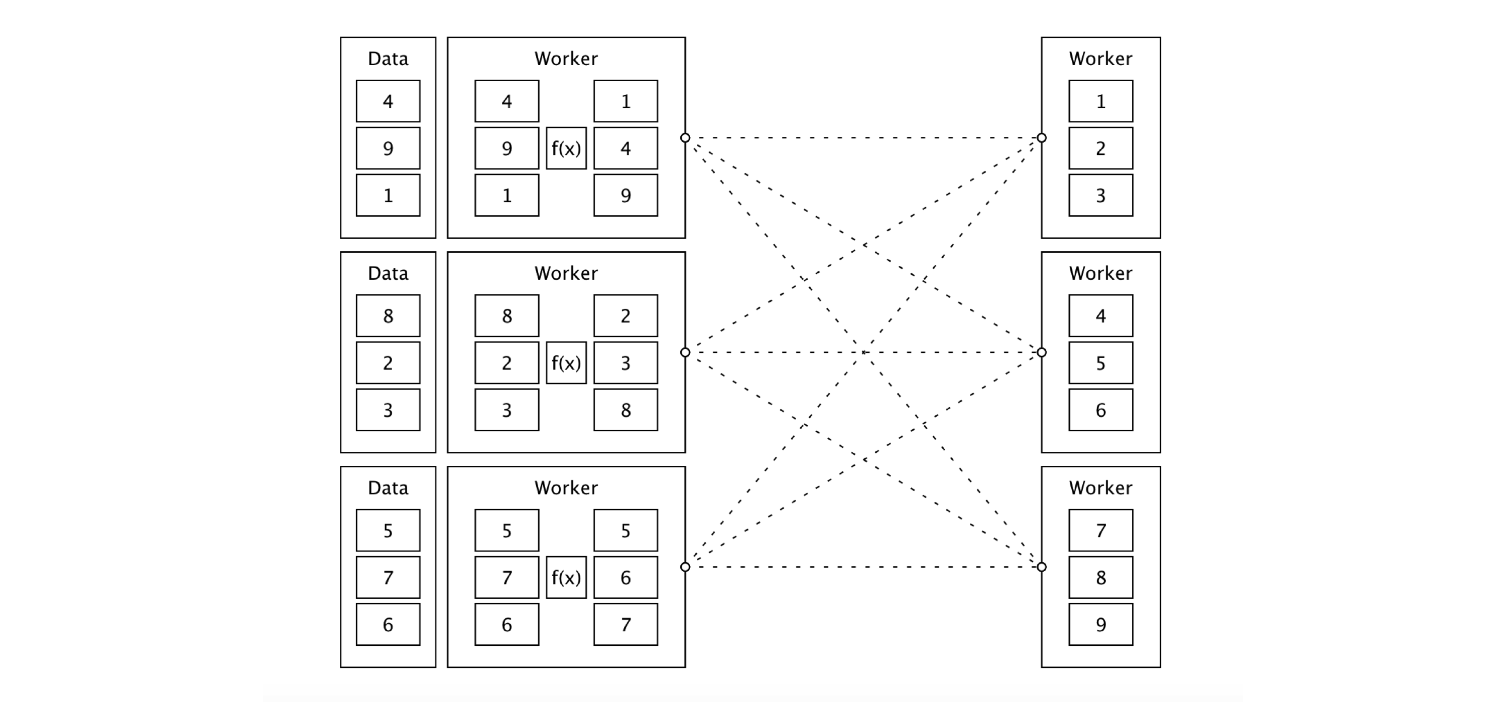
FIGURE 9.1: Sorting distributed data with Apache Spark
9.1.1 Graph
Spark describes all computation steps using a Directed Acyclic Graph (DAG), which means that all computations in Spark move computation forward without repeating previous steps, which helps Spark optimize computations effectively.
The best way to understand Spark’s computation graph for a given operation—sorting for our example—is to open the last completed query on the SQL tab in Spark’s web interface. Figure 9.2 shows the resulting graph for this sorting operation, which contains the following operations:
WholeStageCodegen- This block specifies that the operations it contains were used to generate computer code that was efficiently translated to byte code. There is usually a small cost associated with translating operations into byte code, but this is a worthwhile price to pay since the operations then can be executed much faster from Spark. In general, you can ignore this block and focus on the operations that it contains.
InMemoryTableScan- This means that the original dataset
datawas stored in memory and traversed row by row once. Exchange- Partitions were exchanged—that is, shuffled—across executors in your cluster.
Sort- Once the records arrived at the right executor, they were sorted in this final stage.
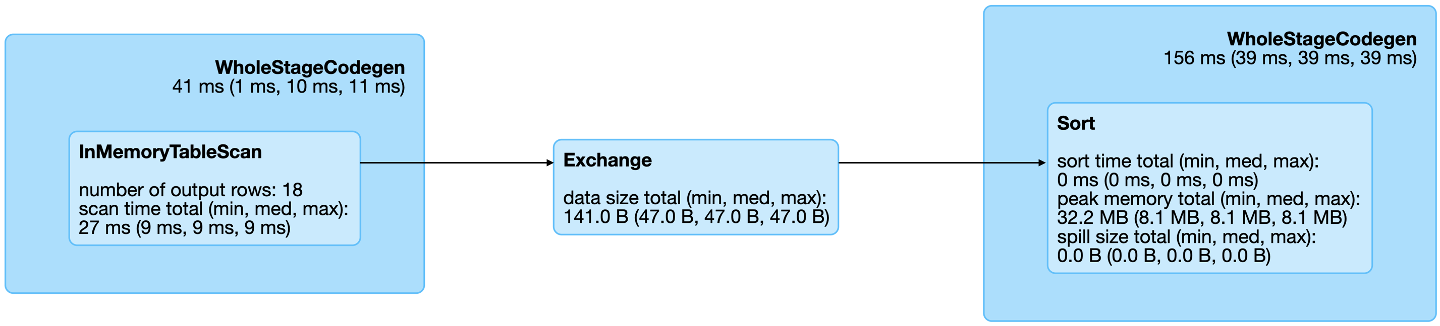
FIGURE 9.2: Spark graph for a sorting query
From the query details, you then can open the last Spark job to arrive to the job details page, which you can expand by using “DAG Visualization” to create a graph similar to Figure 9.3. This graph shows a few additional details and the stages in this job. Notice that there are no arrows pointing back to previous steps, since Spark makes use of acyclic graphs.
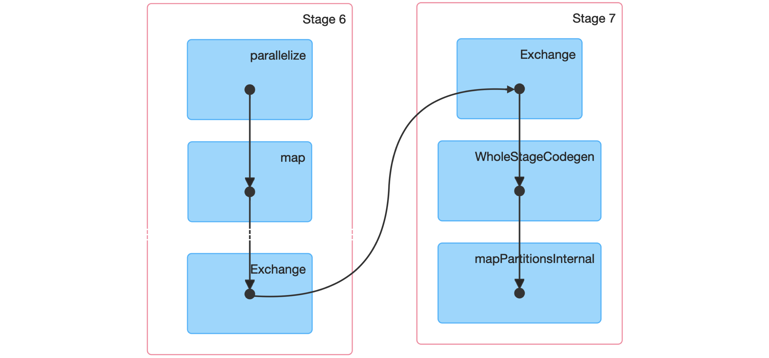
FIGURE 9.3: Spark graph for a sorting job
Next, we dive into a Spark stage and explore its event timeline.
9.1.2 Timeline
The event timeline is a great summary of how Spark is spending computation cycles over each stage. Ideally, you want to see this timeline consisting of mostly CPU usage since other tasks can be considered overhead. You also want to see Spark using all the CPUs across all the cluster nodes available to you.
Select the first stage in the current job and expand the event timeline, which should look similar to Figure 9.4. Notice that we explicitly requested three partitions, which are represented by three lanes in this visualization.
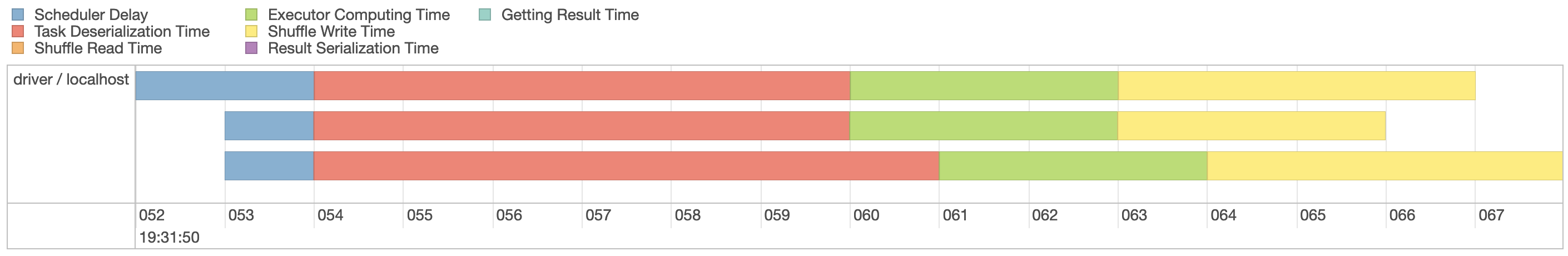
FIGURE 9.4: Spark event timeline
Since our machine is equipped with four CPUs, we can(((“parallel execution”))) parallelize this computation even further by explicitly repartitioning data using sdf_repartition(), with the result shown in Figure 9.5:
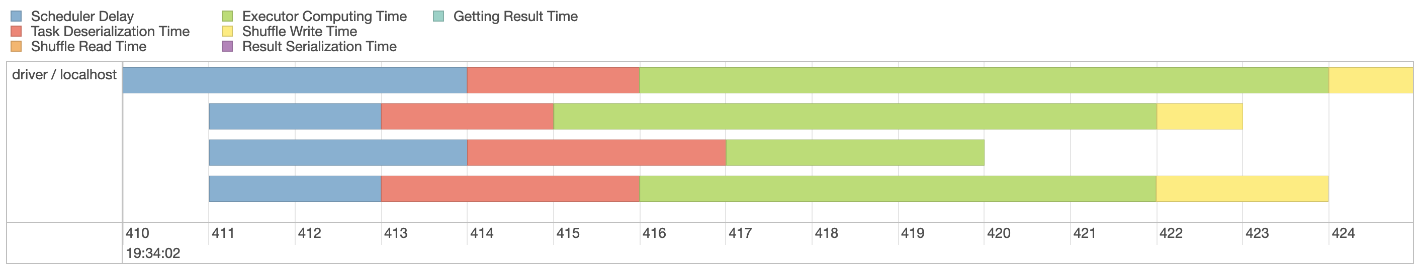
FIGURE 9.5: Spark event timeline with additional partitions
Figure 9.5 now shows four execution lanes with most time spent under Executor Computing Time, which shows us that this particular operation is making better use of our compute resources. When you are working with clusters, requesting more compute nodes from your cluster should shorten computation time. In contrast, for timelines that show significant time spent shuffling, requesting more compute nodes might not shorten time and might actually make everything slower. There is no concrete set of rules to follow to optimize a stage; however, as you gain experience understanding this timeline over multiple operations, you will develop insights as to how to properly optimize Spark operations.
9.2 Configuring
When tuning a Spark application, the most common resources to configure are memory and cores, specifically:
- Memory in driver
- The amount of memory required in the driver node
- Memory per worker
- The amount of memory required in the worker nodes
- Cores per worker
- The number of CPUs required in the worker nodes
- Number of workers
- The number of workers required for this session
Note: It is recommended to request significantly more memory for the driver than the memory available over each worker node. In most cases, you will want to request one core per worker.
In local mode there are no workers, but we can still configure memory and cores to use through the following:
# Initialize configuration with defaults
config <- spark_config()

# Memory
config["sparklyr.shell.driver-memory"] <- "2g"

# Cores
config["sparklyr.connect.cores.local"] <- 2

# Connect to local cluster with custom configuration
sc <- spark_connect(master = "local", config = config)
When using the Spark Standalone and the Mesos cluster managers, all the available memory and cores are assigned by default; therefore, there are no additional configuration changes required, unless you want to restrict resources to allow multiple users to share this cluster. In this case, you can use total-executor-cores to restrict the total executors requested. The Spark Standalone and Spark on Mesos guides provide additional information on sharing clusters.
When running under YARN Client, you would configure memory and cores as follows:
# Memory in Driver
config["sparklyr.shell.driver-memory"] <- "2g"

# Memory per Worker
config["spark.executor.memory"] <- "2G"

# Cores per Worker
config["sparklyr.shell.executor-cores"] <- 1

# Number of Workers
config["sparklyr.shell.num-executors"] <- 3
When using YARN in cluster mode you can use sparklyr.shell.driver-cores to configure total cores requested in the driver node. The Spark on YARN guide provides additional configuration settings that can benefit you.
There are a few types of configuration settings:
- Connect
- These settings are set as parameters to
spark_connect(). They are common settings used while connecting. - Submit
- These settings are set while
sparklyris being submitted to Spark throughspark-submit; some are dependent on the cluster manager being used. - Runtime
- These settings configure Spark when the Spark session is created. They are independent of the cluster manager and specific to Spark.
- sparklyr
- Use these to configure
sparklyrbehavior. These settings are independent of the cluster manager and particular to R.
The following subsections present extensive lists of all the available settings. It is not required that you fully understand them all while tuning Spark, but skimming through them could prove useful in the future for troubleshooting issues. If you prefer, you can skip these subsections and use them instead as reference material as needed.
9.2.1 Connect Settings
You can use the parameters listed in Table 9.1 with spark_connect(). They configure high-level settings that define the connection method, Spark’s installation path, and the version of Spark to use.
| name | value |
|---|---|
| master | Spark cluster url to connect to. Use “local” to connect to a local instance of Spark installed via ‘spark_install()’. |
| spark_home | The path to a Spark installation. Defaults to the path provided by the SPARK_HOME environment variable. If SPARK_HOME is defined, it will always be used unless the version parameter is specified to force the use of a locally installed version. |
| method | The method used to connect to Spark. Default connection method is “shell” to connect using spark-submit, use “livy” to perform remote connections using HTTP, “databricks” when using a Databricks cluster or “qubole” when using a Qubole cluster. |
| app_name | The application name to be used while running in the Spark cluster. |
| version | The version of Spark to use. Only applicable to “local” Spark connections. |
| config | Custom configuration for the generated Spark connection. See spark_config for details. |
You can configure additional settings by specifying a list in the config parameter. Let’s now take a look at what those settings can be.
9.2.2 Submit Settings
Some settings must be specified when spark-submit (the terminal application that launches Spark) is run. For instance, since spark-submit launches a driver node that runs as a Java instance, how much memory is allocated needs to be specified as a parameter to spark-submit.
You can list all the available spark-submit parameters by running the following:
For readability, we’ve provided the output of this command in Table 9.2, replacing the spark-submit parameter with the appropriate spark_config() setting and removing the parameters that are not applicable or already presented in this chapter.
| name | value |
|---|---|
| sparklyr.shell.jars | Specified as ‘jars’ parameter in ‘spark_connect()’. |
| sparklyr.shell.packages | Comma-separated list of maven coordinates of jars to include on the driver and executor classpaths. Will search the local maven repo, then maven central and any additional remote repositories given by ‘sparklyr.shell.repositories’. The format for the coordinates should be groupId:artifactId:version. |
| sparklyr.shell.exclude-packages | Comma-separated list of groupId:artifactId, to exclude while resolving the dependencies provided in ‘sparklyr.shell.packages’ to avoid dependency conflicts. |
| sparklyr.shell.repositories | Comma-separated list of additional remote repositories to search for the maven coordinates given with ‘sparklyr.shell.packages’ |
| sparklyr.shell.files | Comma-separated list of files to be placed in the working directory of each executor. File paths of these files in executors can be accessed via SparkFiles.get(fileName). |
| sparklyr.shell.conf | Arbitrary Spark configuration property set as PROP=VALUE. |
| sparklyr.shell.properties-file | Path to a file from which to load extra properties. If not specified, this will look for conf/spark-defaults.conf. |
| sparklyr.shell.driver-java-options | Extra Java options to pass to the driver. |
| sparklyr.shell.driver-library-path | Extra library path entries to pass to the driver. |
| sparklyr.shell.driver-class-path | Extra class path entries to pass to the driver. Note that jars added with ‘sparklyr.shell.jars’ are automatically included in the classpath. |
| sparklyr.shell.proxy-user | User to impersonate when submitting the application. This argument does not work with ‘sparklyr.shell.principal’ / ‘sparklyr.shell.keytab’. |
| sparklyr.shell.verbose | Print additional debug output. |
The remaining settings, shown in Table 9.3, are specific to YARN.
| name | value |
|---|---|
| sparklyr.shell.queue | The YARN queue to submit to (Default: “default”). |
| sparklyr.shell.archives | Comma separated list of archives to be extracted into the working directory of each executor. |
| sparklyr.shell.principal | Principal to be used to login to KDC, while running on secure HDFS. |
| sparklyr.shell.keytab | The full path to the file that contains the keytab for the principal specified above. This keytab will be copied to the node running the Application Master via the Secure Distributed Cache, for renewing the login tickets and the delegation tokens periodically. |
In general, any spark-submit setting is configured through sparklyr.shell.X, where X is the name of the spark-submit parameter without the -- prefix.
9.2.3 Runtime Settings
As mentioned, some Spark settings configure the session runtime. The runtime settings are a superset of the submit settings given that it is usually helpful to retrieve the current configuration even if a setting can’t be changed.
To list the Spark settings set in your current Spark session, you can run the following:
Table 9.4 describes the runtime settings.
| name | value |
|---|---|
| spark.master | local[4] |
| spark.sql.shuffle.partitions | 4 |
| spark.driver.port | 62314 |
| spark.submit.deployMode | client |
| spark.executor.id | driver |
| spark.jars | /Library/…/sparklyr/java/sparklyr-2.3-2.11.jar |
| spark.app.id | local-1545518234395 |
| spark.env.SPARK_LOCAL_IP | 127.0.0.1 |
| spark.sql.catalogImplementation | hive |
| spark.spark.port.maxRetries | 128 |
| spark.app.name | sparklyr |
| spark.home | /Users/…/spark/spark-2.3.2-bin-hadoop2.7 |
| spark.driver.host | localhost |
However, there are many more configuration settings available in Spark, as described in the Spark Configuration guide. It’s beyond the scope of this book to describe them all, so, if possible, take some time to identify the ones that might be of interest to your particular use cases.
9.2.4 sparklyr Settings
Apart from Spark settings, there are a few settings particular to sparklyr. You usually don’t use these settings while tuning Spark; instead, they are helpful while troubleshooting Spark from R. For instance, you can use sparklyr.log.console = TRUE to output the Spark logs into the R console; this is ideal while troubleshooting but too noisy otherwise. Here’s how to list the settings (results are presented in Table 9.5):
| name | description |
|---|---|
| sparklyr.apply.packages | Configures default value for packages parameter in spark_apply(). |
| sparklyr.apply.rlang | Experimental feature. Turns on improved serialization for spark_apply(). |
| sparklyr.apply.serializer | Configures the version spark_apply() uses to serialize the closure. |
| sparklyr.apply.schema.infer | Number of rows collected to infer schema when column types specified in spark_apply(). |
| sparklyr.arrow | Use Apache Arrow to serialize data? |
| sparklyr.backend.interval | Total seconds sparklyr will check on a backend operation. |
| sparklyr.backend.timeout | Total seconds before sparklyr will give up waiting for a backend operation to complete. |
| sparklyr.collect.batch | Total rows to collect when using batch collection, defaults to 100,000. |
| sparklyr.cancellable | Cancel spark jobs when the R session is interrupted? |
| sparklyr.connect.aftersubmit | R function to call after spark-submit executes. |
| sparklyr.connect.app.jar | The path to the sparklyr jar used in spark_connect(). |
| sparklyr.connect.cores.local | Number of cores to use in spark_connect(master = “local”), defaults to parallel::detectCores(). |
| sparklyr.connect.csv.embedded | Regular expression to match against versions of Spark that require package extension to support CSVs. |
| sparklyr.connect.csv.scala11 | Use Scala 2.11 jars when using embedded CSV jars in Spark 1.6.X. |
| sparklyr.connect.jars | Additional JARs to include while submitting application to Spark. |
| sparklyr.connect.master | The cluster master as spark_connect() master parameter, notice that the ‘spark.master’ setting is usually preferred. |
| sparklyr.connect.packages | Spark packages to include when connecting to Spark. |
| sparklyr.connect.ondisconnect | R function to call after spark_disconnect(). |
| sparklyr.connect.sparksubmit | Command executed instead of spark-submit when connecting. |
| sparklyr.connect.timeout | Total seconds before giving up connecting to the sparklyr gateway while initializing. |
| sparklyr.dplyr.period.splits | Should ‘dplyr’ split column names into database and table? |
| sparklyr.extensions.catalog | Catalog PATH where extension JARs are located. Defaults to ‘TRUE’, ‘FALSE’ to disable. |
| sparklyr.gateway.address | The address of the driver machine. |
| sparklyr.gateway.config.retries | Number of retries to retrieve port and address from config, useful when using functions to query port or address in kubernetes. |
| sparklyr.gateway.interval | Total of seconds sparkyr will check on a gateway connection. |
| sparklyr.gateway.port | The port the sparklyr gateway uses in the driver machine, defaults to 8880. |
| sparklyr.gateway.remote | Should the sparklyr gateway allow remote connections? This is required in yarn cluster, etc. |
| sparklyr.gateway.routing | Should the sparklyr gateway service route to other sessions? Consider disabling in kubernetes. |
| sparklyr.gateway.service | Should the sparklyr gateway be run as a service without shutting down when the last connection disconnects? |
| sparklyr.gateway.timeout | Total seconds before giving up connecting to the sparklyr gateway after initialization. |
| sparklyr.gateway.wait | Total seconds to wait before retrying to contact the sparklyr gateway. |
| sparklyr.livy.auth | Authentication method for Livy connections. |
| sparklyr.livy.headers | Additional HTTP headers for Livy connections. |
| sparklyr.livy.sources | Should sparklyr sources be sourced when connecting? If false, manually register sparklyr jars. |
| sparklyr.log.invoke | Should every call to invoke() be printed in the console? Can be set to ‘callstack’ to log call stack. |
| sparklyr.log.console | Should driver logs be printed in the console? |
| sparklyr.progress | Should job progress be reported to RStudio? |
| sparklyr.progress.interval | Total of seconds to wait before attempting to retrieve job progress in Spark. |
| sparklyr.sanitize.column.names | Should partially unsupported column names be cleaned up? |
| sparklyr.stream.collect.timeout | Total seconds before stopping collecting a stream sample in sdf_collect_stream(). |
| sparklyr.stream.validate.timeout | Total seconds before stopping to check if stream has errors while being created. |
| sparklyr.verbose | Use verbose logging across all sparklyr operations? |
| sparklyr.verbose.na | Use verbose logging when dealing with NAs? |
| sparklyr.verbose.sanitize | Use verbose logging while sanitizing columns and other objects? |
| sparklyr.web.spark | The URL to Spark’s web interface. |
| sparklyr.web.yarn | The URL to YARN’s web interface. |
| sparklyr.worker.gateway.address | The address of the worker machine, most likely localhost. |
| sparklyr.worker.gateway.port | The port the sparklyr gateway uses in the driver machine. |
| sparklyr.yarn.cluster.accepted.timeout | Total seconds before giving up waiting for cluster resources in yarn cluster mode. |
| sparklyr.yarn.cluster.hostaddress.timeout | Total seconds before giving up waiting for the cluster to assign a host address in yarn cluster mode. |
| sparklyr.yarn.cluster.lookup.byname | Should the current user name be used to filter yarn cluster jobs while searching for submitted one? |
| sparklyr.yarn.cluster.lookup.prefix | Application name prefix used to filter yarn cluster jobs while searching for submitted one. |
| sparklyr.yarn.cluster.lookup.username | The user name used to filter yarn cluster jobs while searching for submitted one. |
| sparklyr.yarn.cluster.start.timeout | Total seconds before giving up waiting for yarn cluster application to get registered. |
9.3 Partitioning
As mentioned in Chapter 1, MapReduce and Spark were designed with the purpose of performing computations against data stored across many machines. The subset of the data available for computation over each compute instance is known as a partition.
By default, Spark computes over each existing implicit partition since it’s more effective to run computations where the data is already located. However, there are cases for which you will want to set an explicit partition to help Spark make more efficient use of your cluster resources.
9.3.1 Implicit Partitions
As Chapter 8 explained, Spark can read data stored in many formats and different storage systems; however, since shuffling data is an expensive operation, Spark executes tasks reusing the partitions in the storage system. Therefore, these partitions are implicit to Spark since they are already well defined and expensive to rearrange.
There is always an implicit partition for every computation in Spark defined by the distributed storage system, even for operations which you wouldn’t expect that create partitions, like copy_to().
You can explore the number of partitions a computation will require by using sdf_num_partitions():
[1] 2While in most cases the default partitions work just fine, there are cases for which you will need to be explicit about the partitions you choose.
9.3.2 Explicit Partitions
There will be times when you have many more or far fewer compute instances than data partitions. In both cases, it can help to repartition data to match your cluster resources.
Various data functions, like spark_read_csv(), already support a repartition parameter to request that Spark repartition data appropriately. For instance, we can create a sequence of 10 numbers partitioned by 10 as follows:
[1] 10For datasets that are already partitioned, we can also use sdf_repartition():
[1] 4The number of partitions usually significantly changes the speed and resources being used; for instance, the following example calculates the mean over 10 million rows with different partition sizes:
library(microbenchmark)
library(ggplot2)

microbenchmark(
    "1 Partition(s)" = sdf_len(sc, 10^7, repartition = 1) %>%
      summarise(mean(id)) %>% collect(),
    "2 Partition(s)" = sdf_len(sc, 10^7, repartition = 2) %>%
      summarise(mean(id)) %>% collect(),
    times = 10
) %>% autoplot() + theme_light()
Figure 9.6 shows that sorting data with two partitions is almost twice as fast. This is because two CPUs can be used to execute this operation. However, it is not necessarily the case that higher partitions produce faster computation; instead, partitioning data is particular to your computing cluster and the data analysis operations being performed.
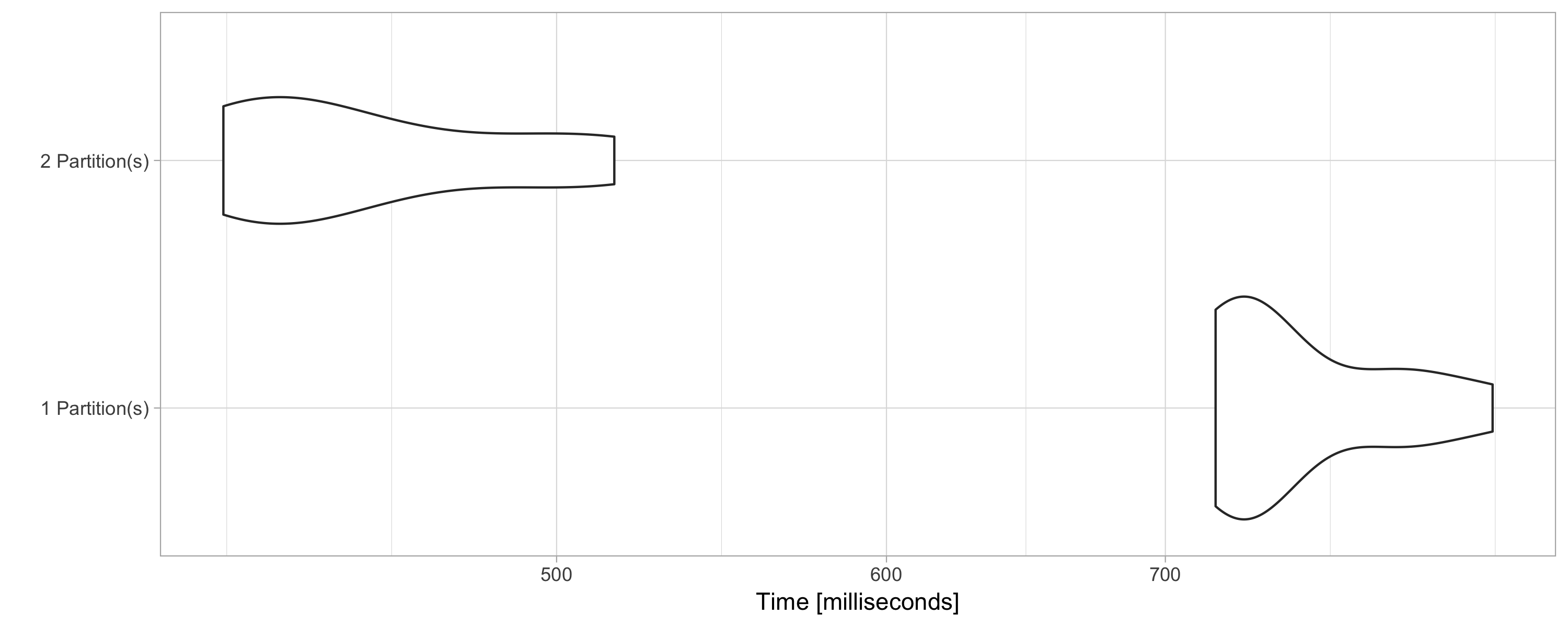
FIGURE 9.6: Computation speed with additional explicit partitions
9.4 Caching
Recall from Chapter 1 that Spark was designed to be faster than its predecessors by using memory instead of disk to store data. This is formally known as a Spark resilient distributed dataset (RDD). An RDD distributes copies of the same data across many machines, such that if one machine fails, others can complete the task—hence, the term “resilient.” Resiliency is important in distributed systems since, while things will usually work in one machine, when running over thousands of machines the likelihood of something failing is much higher. When a failure happens, it is preferable to be fault tolerant to avoid losing the work of all the other machines. RDDs accomplish this by tracking data lineage information to rebuild lost data automatically on failure.
In sparklyr, you can control when an RDD is loaded or unloaded from memory using tbl_cache() and tbl_uncache().
Most sparklyr operations that retrieve a Spark DataFrame cache the results in memory. For instance, running spark_read_parquet() or copy_to() will provide a Spark DataFrame that is already cached in memory. As a Spark DataFrame, this object can be used in most sparklyr functions, including data analysis with dplyr or machine learning:
You can inspect which tables are cached by navigating to the Spark UI using spark_web(sc), clicking the Storage tab, and then clicking on a specific RDD, as illustrated in Figure 9.7.
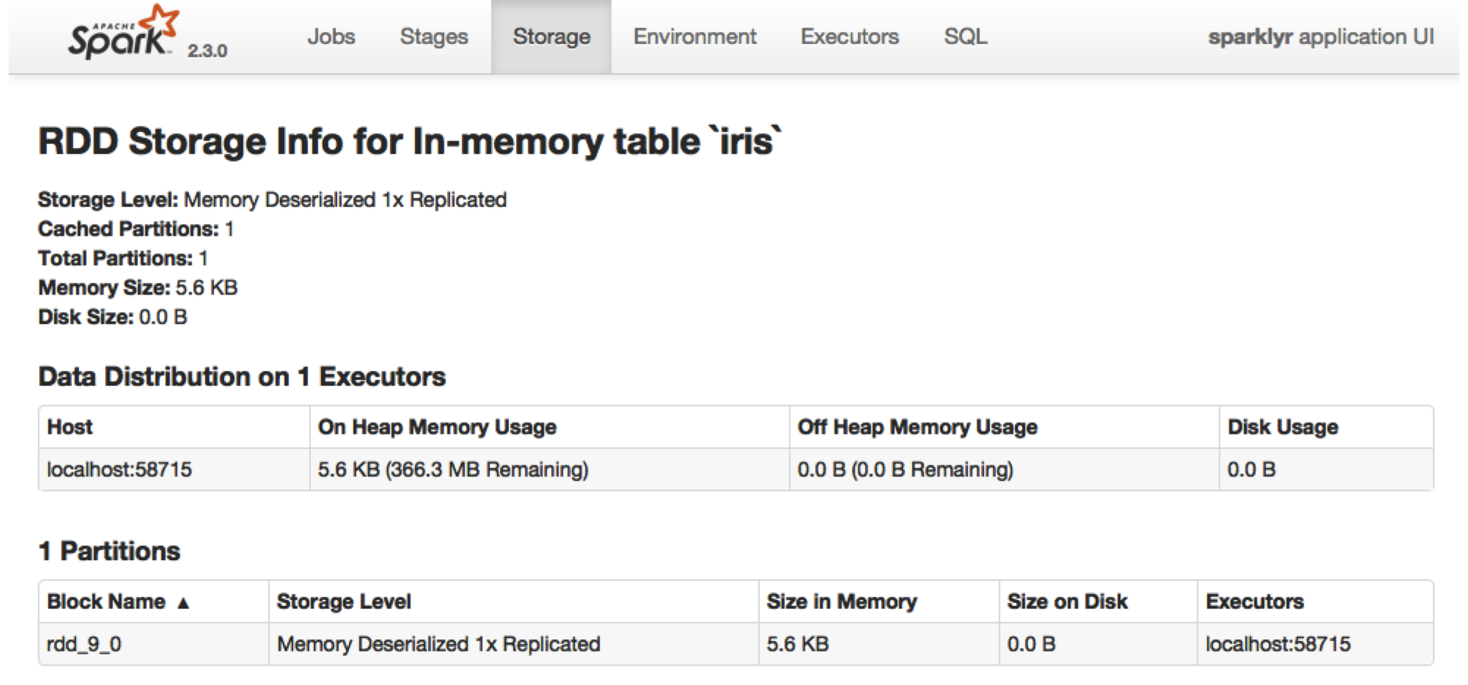
FIGURE 9.7: Cached RDD in the Spark web interface
Data loaded in memory will be released when the R session terminates, either explicitly or implicitly, with a restart or disconnection; however, to free up resources, you can use tbl_uncache():
9.4.1 Checkpointing
Checkpointing is a slightly different type of caching; while it also saves data, it will additionally break the graph computation lineage. For example, if a cached partition is lost, it can be computed from the computation graph, which is not possible with checkpointing since the source of computation is lost.
When performing operations which create expensive computation graphs, it can make sense to checkpoint to save and break the computation lineage in order to help Spark reduce graph computation resources; otherwise, Spark might try to optimize a computation graph that is really not useful to optimize.
You can checkpoint explicitly by saving to CSV, Parquet, and other file formats. Or, let Spark checkpoint this for you by using sdf_checkpoint() in sparklyr, as follows:
# set checkpoint path
spark_set_checkpoint_dir(sc, getwd())

# checkpoint the iris dataset
iris_tbl %>% sdf_checkpoint()
Notice that checkpointing truncates the computation lineage graph, which can speed up performance if the same intermediate result is used multiple times.
9.4.2 Memory
Memory in Spark is categorized into reserved, user, execution, or storage:
- Reserved
- Reserved memory is the memory Spark needs to function and therefore is overhead that is required and should not be configured. This value defaults to 300 MB.
- User
- User memory is the memory used to execute custom code.
sparklyrmakes use of this memory only indirectly when executingdplyrexpressions or modeling a dataset. - Execution
- Execution memory is used to execute code by Spark, mostly to process the results from the partition and perform shuffling.
- Storage
- Storage memory is used to cache RDDs—for instance, when using
compute()insparklyr.
As part of tuning execution, you can consider tweaking the amount of memory allocated for user, execution, and storage by creating a Spark connection with different values than the defaults provided in Spark:
config <- spark_config()

# define memory available for storage and execution
config$spark.memory.fraction <- 0.75

# define memory available for storage
config$spark.memory.storageFraction <- 0.5
For instance, if you want to use Spark to store large amounts of data in memory with the purpose of quickly filtering and retrieving subsets, you can expect Spark to use little execution or user memory. Therefore, to maximize storage memory, you can tune Spark as follows:
config <- spark_config()

# define memory available for storage and execution
config$spark.memory.fraction <- 0.90

# define memory available for storage
config$spark.memory.storageFraction <- 0.90
However, note that Spark will borrow execution memory from storage and vice versa if needed and if possible; therefore, in practice, there should be little need to tune the memory settings.
9.5 Shuffling
Shuffling is the operation that redistributes data across machines; it is usually expensive and therefore something you should try to minimize. You can easily identify whether significant time is being spent shuffling by looking at the event timeline. It is possible to reduce shuffling by reframing data analysis questions or hinting Spark appropriately.
This would be relevant, for instance, when joining DataFrames that differ in size significantly; that is, one set is orders of magnitude smaller than the other one. You can consider using sdf_broadcast() to mark a DataFrame as small enough for use in broadcast joins, meaning it pushes one of the smaller DataFrames to each of the worker nodes to reduce shuffling the bigger DataFrame. Here’s one example for sdf_broadcast():
9.6 Serialization
Serialization is the process of translating data and tasks into a format that can be transmitted between machines and reconstructed on the receiving end.
It is not that common to need to adjust serialization when tuning Spark; however, it is worth mentioning that there are alternative serialization modules like the Kryo Serializer that can provide performance improvements over the default Java Serializer.
You can turn on the Kryo Serializer in sparklyr through the following:
9.7 Configuration Files
Configuring the spark_config() settings before connecting is the most common approach while tuning Spark. However, after you identify the parameters in your connection, you should consider switching to use a configuration file since it will remove the clutter in your connection code and also allow you to share the configuration settings across projects and coworkers.
For instance, instead of connecting to Spark like this:
config <- spark_config()
config["sparklyr.shell.driver-memory"] <- "2G"
sc <- spark_connect(master = "local", config = config)
you can define a config.yml file with the desired settings. This file should be located in the current working directory or in parent directories. For example, you can create the following config.yml file to modify the default driver memory:
Then, connecting with the same configuration settings becomes much cleaner by using instead:
You can also specify an alternate configuration filename or location by setting the file parameter in spark_config(). One additional benefit from using configuration files is that a system administrator can change the default configuration by changing the value of the R_CONFIG_ACTIVE environment variable. See the GitHub rstudio/config repo for additional information.
9.8 Recap
This chapter provided a broad overview of Spark internals and detailed configuration settings to help you speed up computation and enable high computation loads. It provided the foundations to understand bottlenecks and guidance on common configuration considerations. However, fine-tuning Spark is a broad topic that would require many more chapters to cover extensively. Therefore, while troubleshooting Spark’s performance and scalability, searching the web, and consulting online communities, it is often necessary to fine-tune your particular environment as well.
Chapter 10 introduces the ecosystem of Spark extensions that are available in R. Most extensions are highly specialized, but they will prove to be extremely useful in specific cases and for readers with particular needs. For instance, they can process nested data, perform graph analysis, and use different modeling libraries like rsparkling from H20. In addition, the next few chapters introduce many advanced data analysis and modeling topics that are required to master large-scale computing in R.