Chapter 12 Streaming
Our stories aren’t over yet.
— Arya Stark
Looking back at the previous chapters, we’ve covered a good deal, but not everything. We’ve analyzed tabular datasets, performed unsupervised learning over raw text, analyzed graphs and geographic datasets, and even transformed data with custom R code! So now what?
Though we weren’t explicit about this, we’ve assumed until this point that your data is static, and didn’t change over time. But suppose for a moment your job is to analyze traffic patterns to give recommendations to the department of transportation. A reasonable approach would be to analyze historical data and then design predictive models that compute forecasts overnight. Overnight? That’s very useful, but traffic patterns change by the hour and even by the minute. You could try to preprocess and predict faster and faster, but eventually this model breaks—you can’t load large-scale datasets, transform them, score them, unload them, and repeat this process by the second.
Instead, we need to introduce a different kind of dataset—one that is not static but rather dynamic, one that is like a table but is growing constantly. We will refer to such datasets as streams.
12.1 Overview
We know how to work with large-scale static datasets, but how can we reason about large-scale real-time datasets? Datasets with an infinite amount of entries are known as streams.
For static datasets, if we were to do real-time scoring using a pretrained topic model, the entries would be lines of text; for real-time datasets, we would perform the same scoring over an infinite number of lines of text. Now, in practice, you will never process an infinite number of records. You will eventually stop the stream—or this universe might end, whichever comes first. Regardless, thinking of the datasets as infinite makes it much easier to reason about them.
Streams are most relevant when processing real-time data—for example, when analyzing a Twitter feed or stock prices. Both examples have well-defined columns, like “tweet” or “price,” but there are always new rows of data to be analyzed.
Spark Streaming provides scalable and fault-tolerant data processing over streams of data. That means you can use many machines to process multiple streaming sources, perform joins with other streams or static sources, and recover from failures with at-least-once guarantees (each message is certain to be delivered, but may do so multiple times).
In Spark, you create streams by defining a source, a transformation, and a sink; you can think of these steps as reading, transforming, and writing a stream, as shown in Figure 12.1 describes.
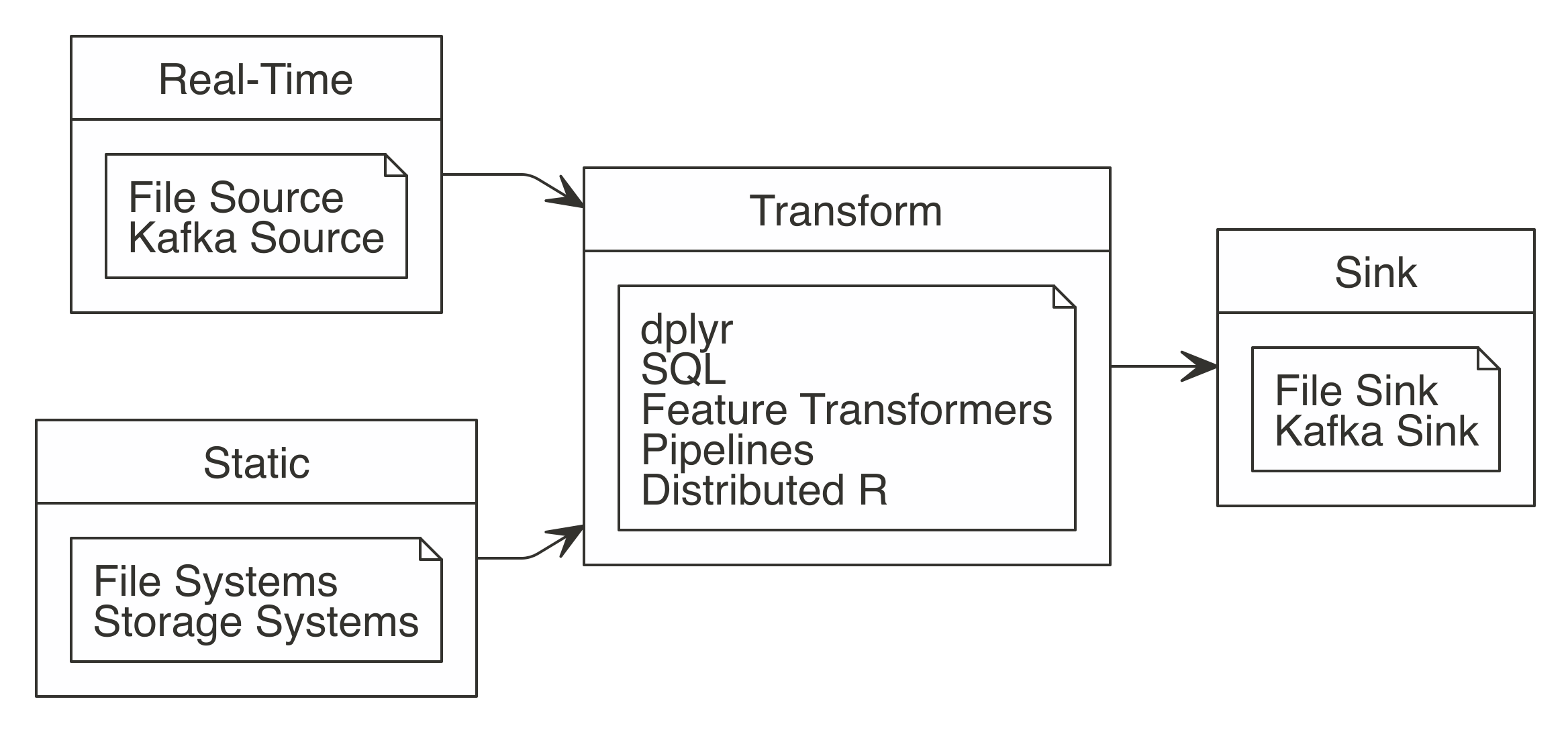
FIGURE 12.1: Working with Spark Streaming
Let’s take a look at each of these a little more closely:
- Reading
- Streams read data using any of the
stream_read_*()functions; the read operation defines the source of the stream. You can define one or multiple sources from which to read. - Transforming
- A stream can perform one or multiple transformations using
dplyr,SQL, feature transformers, scoring pipelines, or distributed R code. Transformations can not only be applied to one or more streams, but can also use a combination of streams and static data sources; for instance, those loaded into Spark withspark_read_()functions—this means that you can combine static data and real-time data sources with ease. - Writing
- The write operations are performed with the family of
stream_write_*()functions, while the read operation defined the sink of the stream. You can specify a single sink or multiple ones to write data to.
You can read and write to streams in several different file formats: CSV, JSON, Parquet, Optimized Row Columnar (ORC), and text (see Table 12.1). You also can read and write from and to Kafka, which we will introduce later on.
| Format | Read | Write |
|---|---|---|
| CSV | stream_read_csv | stream_write_csv |
| JSON | stream_read_json | stream_write_json |
| Kafka | stream_read_kafka | stream_write_kafka |
| ORC | stream_read_orc | stream_write_orc |
| Parquet | stream_read_parquet | stream_write_parquet |
| Text | stream_read_text | stream_write_text |
| Memory | stream_write_memory |
Since the transformation step is optional, the simplest stream we can define is one that continuously copies text files between source and destination.
First, install the future package using install.packages("future") and connect to Spark.
Since a stream requires the source to exist, create a source folder:
We are now ready to define our first stream!
The streams starts running with stream_write_*(); once executed, the stream will monitor the source path and process data into the ++destination /++ path as it arrives.
We can use stream_generate_test() to produce a file every second containing lines of text that follow a given distribution; you can read more about this in Appendix. In practice, you would connect to existing sources without having to generate data artificially. We can then use view_stream() to track the rows per second (rps) being processed in the source, and in the destination, and their latest values over time:
The result is shown in Figure 12.2.
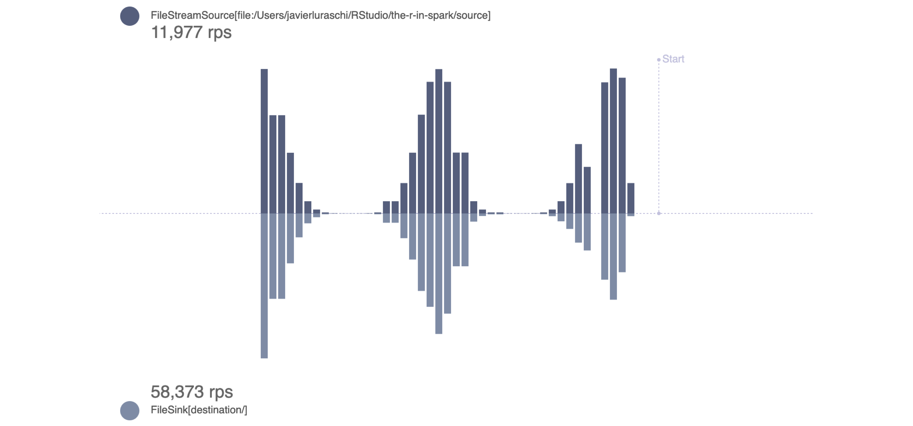
FIGURE 12.2: Monitoring a stream generating rows following a binomial distribution
Notice that the rps rate in the destination stream is higher than that in the source stream. This is expected and desirable since Spark measures incoming rates from the source stream, but also actual row-processing times in the destination stream. For example, if 10 rows per second are written to the source/ path, the incoming rate is 10 rps. However, if it takes Spark only 0.01 seconds to write all those 10 rows, the output rate is 100 rps.
Use stream_stop() to properly stop processing data from this stream:
This exercise introduced how we can easily start a Spark stream that reads and writes data based on a simulated stream. Let’s do something more interesting than just copying data with proper transformations.
12.2 Transformations
In a real-life scenario, the incoming data from a stream would not be written as is to the output. The Spark Streaming job would make transformations to the data, and then write the transformed data.
Streams can be transformed using dplyr, SQL queries, ML pipelines, or R code. We can use as many transformations as needed in the same way that Spark DataFrames can be transformed with sparklyr.
The source of the transformation can be a stream or DataFrame, but the output is always a stream. If needed, you can always take a snapshot from the destination stream and then save the output as a DataFrame. That is what sparklyr will do for you if a destination stream is not specified.
Each of the following subsections covers an option provided by sparklyr to perform transformations on a stream.
12.2.1 Analysis
You can analyze streams with dplyr verbs and SQL using DBI. As a quick example, we will filter rows and add columns over a stream. We won’t explicitly call stream_generate_test(), but you can call it on your own through the later package if you feel the urge to verify that data is being processed continuously:
# Source: spark<?> [inf x 2]
       x     y
   <int> <dbl>
 1   701     7
 2   702     7
 3   703     7
 4   704     7
 5   705     7
 6   706     7
 7   707     7
 8   708     7
 9   709     7
10   710     7
# … with more rows
It’s also possible to perform aggregations over the entire history of the stream. The history could be filtered or not:
# Source: spark<?> [inf x 2]
      y     n
  <dbl> <dbl>
1     8 25902
2     9 25902
3    10 13210
4     7 12692
Grouped aggregations of the latest data in the stream require a timestamp. The timestamp will note when the reading function (in this case stream_read_csv()) first “saw” that specific record. In Spark Streaming terminology, the timestamp is called a watermark. The spark_watermark() function adds the timestamp. In this example, the watermark will be the same for all records, since the five files were read by the stream after they were created. Note that only Kafka and memory outputs support watermarks:
# Source: spark<?> [inf x 2]
x timestamp
<int> <dttm>
1 276 2019-06-30 07:14:21
2 277 2019-06-30 07:14:21
3 278 2019-06-30 07:14:21
4 279 2019-06-30 07:14:21
5 280 2019-06-30 07:14:21
6 281 2019-06-30 07:14:21
7 282 2019-06-30 07:14:21
8 283 2019-06-30 07:14:21
9 284 2019-06-30 07:14:21
10 285 2019-06-30 07:14:21
# … with more rowsAfter the watermark is created, you can use it in the group_by() verb. You can then pipe it into a summarise() function to get some stats of the stream:
stream_read_csv(sc, "source") %>%
stream_watermark() %>%
group_by(timestamp) %>%
summarise(
max_x = max(x, na.rm = TRUE),
min_x = min(x, na.rm = TRUE),
count = n()
) # Source: spark<?> [inf x 4]
timestamp max_x min_x count
<dttm> <int> <int> <dbl>
1 2019-06-30 07:14:55 1000 1 25933212.2.2 Modeling
Spark streams currently don’t support training on real-time datasets. Aside from the technical challenges, even if it were possible, it would be quite difficult to train models since the model itself would need to adapt over time. Known as online learning, this is perhaps something that Spark will support in the future.
That said, there are other modeling concepts we can use with streams, like feature transformers and scoring. Let’s try out a feature transformer with streams, and leave scoring for the next section, since we will need to train a model.
The next example uses the ft_bucketizer() feature transformer to modify the stream followed by regular dplyr functions, which you can use just as you would with static datasets:
stream_read_csv(sc, "source") %>%
  mutate(x = as.numeric(x)) %>%
  ft_bucketizer("x", "buckets", splits = 0:10 * 100) %>%
  count(buckets)  %>%
  arrange(buckets)
# Source: spark<?> [inf x 2]
# Ordered by: buckets
buckets n
<dbl> <dbl>
1 0 25747
2 1 26008
3 2 25992
4 3 25908
5 4 25905
6 5 25903
7 6 25904
8 7 25901
9 8 25902
10 9 2616212.2.3 Pipelines
Spark pipelines can be used for scoring streams, but not to train over streaming data. The former is fully supported, while the latter is a feature under active development by the Spark community.
To score a stream, it’s necessary to first create our model. So let’s build, fit, and save a simple pipeline:
cars <- copy_to(sc, mtcars)

model <- ml_pipeline(sc) %>%
  ft_binarizer("mpg", "over_30", 30) %>%
  ft_r_formula(over_30 ~ wt) %>%
  ml_logistic_regression() %>%
  ml_fit(cars)
Tip: If you choose to, you can make use of other concepts presented in Chapter 5, like saving and reloading pipelines through ml_save() and ml_load() before scoring streams.
We can then generate a stream based on mtcars using stream_generate_test(), and score the model using ml_transform():
future::future(stream_generate_test(mtcars, "cars-stream", iterations = 5))

ml_transform(model, stream_read_csv(sc, "cars-stream"))
# Source: spark<?> [inf x 17]
mpg cyl disp hp drat wt qsec vs am gear carb over_30
<dbl> <int> <dbl> <int> <dbl> <dbl> <dbl> <int> <int> <int> <int> <dbl>
1 15.5 8 318 150 2.76 3.52 16.9 0 0 3 2 0
2 15.2 8 304 150 3.15 3.44 17.3 0 0 3 2 0
3 13.3 8 350 245 3.73 3.84 15.4 0 0 3 4 0
4 19.2 8 400 175 3.08 3.84 17.0 0 0 3 2 0
5 27.3 4 79 66 4.08 1.94 18.9 1 1 4 1 0
6 26 4 120. 91 4.43 2.14 16.7 0 1 5 2 0
7 30.4 4 95.1 113 3.77 1.51 16.9 1 1 5 2 1
8 15.8 8 351 264 4.22 3.17 14.5 0 1 5 4 0
9 19.7 6 145 175 3.62 2.77 15.5 0 1 5 6 0
10 15 8 301 335 3.54 3.57 14.6 0 1 5 8 0
# … with more rows, and 5 more variables: features <list>, label <dbl>,
# rawPrediction <list>, probability <list>, prediction <dbl>Though this example was put together with a few lines of code, what we just accomplished is actually quite impressive. You copied data into Spark, performed feature engineering, trained a model, and scored the model over a real-time dataset, with just seven lines of code! Let’s try now to use custom transformations, in real time.
12.2.4 Distributed R {streaming-r-code}
Arbitrary R code can also be used to transform a stream with the use of spark_apply(). This approach follows the same principles discussed in Chapter 11, where spark_apply() runs R code over each executor in the cluster where data is available. This enables processing high-throughput streams and fulfills low-latency requirements:
stream_read_csv(sc, "cars-stream") %>%
  select(mpg) %>%
  spark_apply(~ round(.x), mpg = "integer") %>%
  stream_write_csv("cars-round")
which, as you would expect, processes data from cars-stream into cars-round by running the custom round() R function. Let’s peek into the output sink:
# Source: spark<carsround> [?? x 1]
     mpg
   <dbl>
 1    16
 2    15
 3    13
 4    19
 5    27
 6    26
 7    30
 8    16
 9    20
10    15
# … with more rows
Again, make sure you apply the concepts you already know about spark_apply() when using streams; for instance, you should consider using arrow to significantly improve performance. Before we move on, disconnect from Spark:
This was our last transformation for streams. We’ll now learn how to use Spark Streaming with Kafka.
12.3 Kafka
Apache Kafka is an open source stream-processing software platform developed by LinkedIn and donated to the Apache Software Foundation. It is written in Scala and Java. To describe it using an analogy, Kafka is to real-time storage what Hadoop is to static storage.
Kafka stores the stream as records, which consist of a key, a value, and a timestamp. It can handle multiple streams that contain different information, by categorizing them by topic. Kafka is commonly used to connect multiple real-time applications. A producer is an application that streams data into Kafka, while a consumer is the one that reads from Kafka; in Kafka terminology, a consumer application subscribes to topics. Therefore, the most basic workflow we can accomplish with Kafka is one with a single producer and a single consumer; this is illustrated in Figure 12.3.
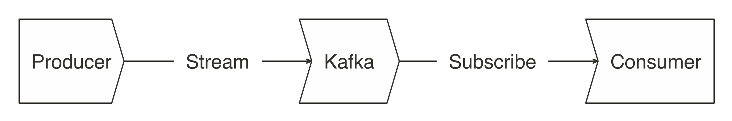
FIGURE 12.3: A basic Kafka workflow
If you are new to Kafka, we don’t recommend you run the code from this section. However, if you’re really motivated to follow along, you will first need to install Kafka as explained in Appendix or deploy it in your cluster.
Using Kafka also requires you to have the Kafka package when connecting to Spark. Make sure this is specified in your connection config:
library(sparklyr)
library(dplyr)

sc <- spark_connect(master = "local", config = list(
  sparklyr.shell.packages = "org.apache.spark:spark-sql-kafka-0-10_2.11:2.4.0"
))
Once connected, it’s straightforward to read data from a stream:
stream_read_kafka(
  sc,
  options = list(
    kafka.bootstrap.server = "host1:9092, host2:9092",
    subscribe = "<topic-name>"
    )
  )
However, notice that you need to properly configure the options list; kafka.bootstrap.server expects a list of Kafka hosts, while topic and subscribe define which topic should be used when writing or reading from Kafka, respectively.
Though we’ve started by presenting a simple single-producer and single-consumer use case, Kafka also allows much more complex interactions. We will next read from one topic, process its data, and then write the results to a different topic. Systems that are producers and consumers from the same topic are referred to as stream processors. In Figure 12.4, the stream processor reads topic A and then writes results to topic B. This allows for a given consumer application to read results instead of “raw” feed data.
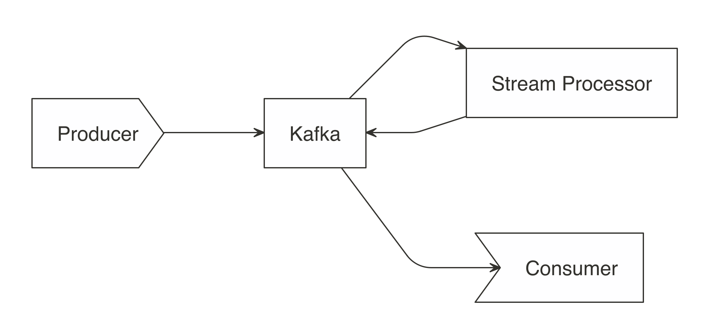
FIGURE 12.4: A Kafka workflow using stream processors
Three modes are available when processing Kafka streams in Spark: complete, update, and append. The complete mode provides the totals for every group every time there is a new batch; update provides totals for only the groups that have updates in the latest batch; and append adds raw records to the target topic. The append mode is not meant for aggregates, but works well for passing a filtered subset to the target topic.
In our next example, the producer streams random letters into Kafka under a letters topic. Then, Spark will act as the stream processor, reading the letters topic and computing unique letters, which are then written back to Kafka under the totals topic. We’ll use the update mode when writing back into Kafka; that is, only the totals that changed will be sent to Kafka. This change is determined after each batch from the letters topic:
hosts  <- "localhost:9092"

read_options <- list(kafka.bootstrap.servers = hosts, subscribe = "letters")
write_options <- list(kafka.bootstrap.servers = hosts, topic = "totals")

stream_read_kafka(sc, options = read_options) %>%
  mutate(value = as.character(value)) %>%         # coerce into a character
  count(value) %>%                                # group and count letters
  mutate(value = paste0(value, "=", n)) %>%       # kafka expects a value field
  stream_write_kafka(mode = "update",
                     options = write_options)
You can take a quick look at totals by reading from Kafka:
Using a new terminal session, use Kafka’s command-line tool to manually add single letters into the letters topic:
kafka-console-producer.sh --broker-list localhost:9092 --topic letters
>A
>B
>C
The letters that you input are pushed to Kafka, read by Spark, aggregated within Spark, and pushed back into Kafka, Then, finally, they are consumed by Spark again to give you a glimpse into the totals topic. This was quite a setup, but also a realistic configuration commonly found in real-time processing projects.
Next, we will use the Shiny framework to visualize streams, in real time!
12.4 Shiny
Shiny’s reactive framework is well suited to support streaming information, which you can use to display real-time data from Spark using reactiveSpark(). There is far more to learn about Shiny than we could possibly present here. However, if you’re already familiar with Shiny, this example should be quite easy to understand.
We have a modified version of the k-means Shiny example that, instead of getting the data from the static iris dataset, is generated with stream_generate_test(), consumed by Spark, retrieved to Shiny through reactiveSpark(), and then displayed as shown in Figure 12.5.
To run this example, store the following Shiny app under shiny/shiny-stream.R:
library(sparklyr)
library(shiny)

unlink("shiny-stream", recursive = TRUE)
dir.create("shiny-stream", showWarnings = FALSE)

sc <- spark_connect(
  master = "local", version = "2.3",
  config = list(sparklyr.sanitize.column.names = FALSE))

ui <- pageWithSidebar(
  headerPanel('Iris k-means clustering from Spark stream'),
  sidebarPanel(
    selectInput('xcol', 'X Variable', names(iris)),
    selectInput('ycol', 'Y Variable', names(iris),
                selected=names(iris)[[2]]),
    numericInput('clusters', 'Cluster count', 3,
                 min = 1, max = 9)
  ),
  mainPanel(plotOutput('plot1'))
)

server <- function(input, output, session) {
  iris <- stream_read_csv(sc, "shiny-stream",
                          columns = sapply(datasets::iris, class)) %>%
    reactiveSpark()

  selectedData <- reactive(iris()[, c(input$xcol, input$ycol)])
  clusters <- reactive(kmeans(selectedData(), input$clusters))

  output$plot1 <- renderPlot({
    par(mar = c(5.1, 4.1, 0, 1))
    plot(selectedData(), col = clusters()$cluster, pch = 20, cex = 3)
    points(clusters()$centers, pch = 4, cex = 4, lwd = 4)
  })
}

shinyApp(ui, server)
This Shiny application can then be launched with runApp(), like so:
While the Shiny app is running, launch a new R session from the same directory and create a test stream with stream_generate_test(). This will generate a stream of continuous data that Spark can process and Shiny can visualize (as illustrated in Figure 12.5):
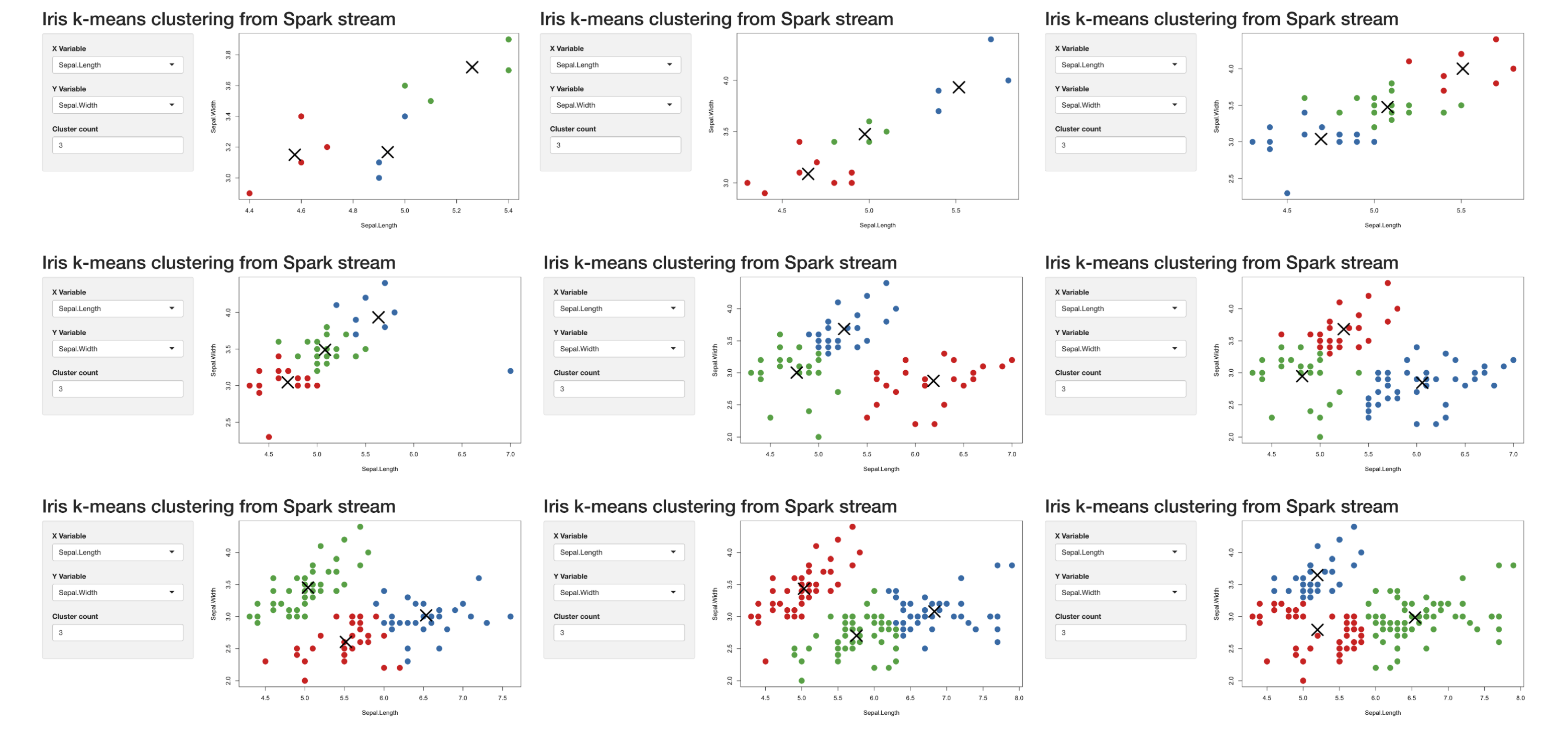
FIGURE 12.5: Progression of Spark reactive loading data into the Shiny app
In this section you learned how easy it is to create a Shiny app that can be used for several different purposes, such as monitoring and dashboarding.
In a more complex implementation, the source would more likely be a Kafka stream.
Before we transition, disconnect from Spark and clear the folders that we used:
12.5 Recap
From static datasets to real-time datasets, you’ve truly mastered many of the large-scale computing techniques. Specifically, in this chapter, you learned how static data can be generalized to real time if we think of it as an infinite table. We were then able to create a simple stream, without any data transformations, that copies data from point A to point B.
This humble start became quite useful when you learned about the several different transformations you can apply to streaming data—from data analysis transformations using the dplyr and DBI packages, to feature transformers introduced while modeling, to fully fledged pipelines capable of scoring in real time, to, last but not least, transforming datasets with custom R code. This was a lot to digest, for sure.
We then presented Apache Kafka as a reliable and scalable solution for real-time data. We showed you how a real-time system could be structured by introducing you to consumers, producers, and topics. These, when properly combined, create powerful abstractions to process real-time data.
Then we closed with “a cherry on top of the sundae”: presenting how to use Spark Streaming in Shiny. Since a stream can be transformed into a reactive (which is the lingua franca of the world of reactivity), the ease of this approach was a nice surprise.
It’s time now to move on to our very last (and quite short) chapter, Chapter 13; there we’ll try to persuade you to use your newly acquired knowledge for the benefit of the Spark and R communities at large.