Chapter 2 Getting Started
I always wanted to be a wizard.
— Samwell Tarly
After reading Chapter 1, you should now be familiar with the kinds of problems that Spark can help you solve. And it should be clear that Spark solves problems by making use of multiple computers when data does not fit in a single machine or when computation is too slow. If you are newer to R, it should also be clear that combining Spark with data science tools like ggplot2 for visualization and dplyr to perform data transformations brings a promising landscape for doing data science at scale. We also hope you are excited to become proficient in large-scale computing.
In this chapter, we take a tour of the tools you’ll need to become proficient in Spark. We encourage you to walk through the code in this chapter because it will force you to go through the motions of analyzing, modeling, reading, and writing data. In other words, you will need to do some wax-on, wax-off, repeat before you get fully immersed in the world of Spark.
In Chapter 3 we dive into analysis followed by modeling, which presents examples using a single-cluster machine: your personal computer. Subsequent chapters introduce cluster computing and the concepts and techniques that you’ll need to successfully run code across multiple machines.
2.1 Overview
From R, getting started with Spark using sparklyr and a local cluster is as easy as installing and loading the sparklyr package followed by installing Spark using sparklyr however, we assume you are starting with a brand new computer running Windows, macOS, or Linux, so we’ll walk you through the prerequisites before connecting to a local Spark cluster.
Although this chapter is designed to help you get ready to use Spark on your personal computer, it’s also likely that some readers will already have a Spark cluster available or might prefer to get started with an online Spark cluster. For instance, Databricks hosts a free community edition of Spark that you can easily access from your web browser. If you end up choosing this path, skip to Prerequisites, but make sure you consult the proper resources for your existing or online Spark cluster.
Either way, after you are done with the prerequisites, you will first learn how to connect to Spark. We then present the most important tools and operations that you’ll use throughout the rest of this book. Less emphasis is placed on teaching concepts or how to use them—we can’t possibly explain modeling or streaming in a single chapter. However, going through this chapter should give you a brief glimpse of what to expect and give you the confidence that you have the tools correctly configured to tackle more challenging problems later on.
The tools you’ll use are mostly divided into R code and the Spark web interface. All Spark operations are run from R; however, monitoring execution of distributed operations is performed from Spark’s web interface, which you can load from any web browser. We then disconnect from this local cluster, which is easy to forget to do but highly recommended while working with local clusters—and in shared Spark clusters as well!
We close this chapter by walking you through some of the features that make using Spark with RStudio easier; more specifically, we present the RStudio extensions that sparklyr implements. However, if you are inclined to use Jupyter Notebooks or if your cluster is already equipped with a different R user interface, rest assured that you can use Spark with R through plain R code. Let’s move along and get your prerequisites properly configured.
2.2 Prerequisites
R can run in many platforms and environments; therefore, whether you use Windows, Mac, or Linux, the first step is to install R from r-project.org; detailed instructions are provided in Installing R.
Most people use programming languages with tools to make them more productive; for R, RStudio is such a tool. Strictly speaking, RStudio is an integrated development environment (IDE), which also happens to support many platforms and environments. We strongly recommend you install RStudio if you haven’t done so already; see details in Using RStudio.
Tip: When using Windows, we recommend avoiding directories with spaces in their path. If running getwd() from R returns a path with spaces, consider switching to a path with no spaces using setwd("path") or by creating an RStudio project in a path with no spaces.
Additionally, because Spark is built in the Scala programming language, which is run by the Java Virtual Machine (JVM), you also need to install Java 8 on your system. It is likely that your system already has Java installed, but you should still check the version and update or downgrade as described in Installing Java. You can use the following R command to check which version is installed on your system:
java version "1.8.0_201"
Java(TM) SE Runtime Environment (build 1.8.0_201-b09)
Java HotSpot(TM) 64-Bit Server VM (build 25.201-b09, mixed mode)
You can also use the JAVA_HOME environment variable to point to a specific Java version by running Sys.setenv(JAVA_HOME = "path-to-java-8"); either way, before moving on to installing sparklyr, make sure that Java 8 is the version available for R.
2.2.1 Installing sparklyr
As with many other R packages, you can install sparklyr from CRAN as follows:
The examples in this book assume you are using the latest version of sparklyr. You can verify your version is as new as the one we are using by running the following:
[1] ‘1.0.2’2.2.2 Installing Spark
Start by loading sparklyr:
This makes all sparklyr functions available in R, which is really helpful; otherwise, you would need to run each sparklyr command prefixed with sparklyr::.
You can easily install Spark by running spark_install(). This downloads, installs, and configures the latest version of Spark locally on your computer; however, because we’ve written this book with Spark 2.3, you should also install this version to make sure that you can follow all the examples provided without any surprises:
You can display all of the versions of Spark that are available for installation by running the following:
##   spark
## 1   1.6
## 2   2.0
## 3   2.1
## 4   2.2
## 5   2.3
## 6   2.4
You can install a specific version by using the Spark version and, optionally, by also specifying the Hadoop version. For instance, to install Spark 1.6.3, you would run:
You can also check which versions are installed by running this command:
  spark hadoop                              dir
7 2.3.1    2.7 /spark/spark-2.3.1-bin-hadoop2.7
The path where Spark is installed is known as Spark’s home, which is defined in R code and system configuration settings with the SPARK_HOME identifier. When you are using a local Spark cluster installed with sparklyr, this path is already known and no additional configuration needs to take place.
Finally, to uninstall a specific version of Spark you can run spark_uninstall() by specifying the Spark and Hadoop versions, like so:
Note: The default installation paths are ~/spark for macOS and Linux, and %LOCALAPPDATA%/spark for Windows. To customize the installation path, you can run options(spark.install.dir = "installation-path") before spark_install() and spark_connect().
2.3 Connecting
It’s important to mention that, so far, we’ve installed only a local Spark cluster. A local cluster is really helpful to get started, test code, and troubleshoot with ease. Later chapters explain where to find, install, and connect to real Spark clusters with many machines, but for the first few chapters, we focus on using local clusters.
To connect to this local cluster, simply run the following:
Note: If you are using your own or online Spark cluster, make sure that you connect as specified by your cluster administrator or the online documentation. If you need some pointers, you can take a quick look at Chapter 7, which explains in detail how to connect to any Spark cluster.
The master parameter identifies which is the “main” machine from the Spark cluster; this machine is often called the driver node. While working with real clusters using many machines, you’ll find that most machines will be worker machines and one will be the master. Since we have only a local cluster with just one machine, we will default to using "local" for now.
After a connection is established, spark_connect() retrieves an active Spark connection, which most code usually names sc; you will then make use of sc to execute Spark commands.
If the connection fails, Chapter 7 contains a troubleshooting section that can help you to resolve your connection issue.
2.4 Using Spark
Now that you are connected, we can run a few simple commands. For instance, let’s start by copying the mtcars dataset into Apache Spark by using copy_to():
The data was copied into Spark, but we can access it from R using the cars reference. To print its contents, we can simply type *cars*:
# Source: spark<mtcars> [?? x 11]
     mpg   cyl  disp    hp  drat    wt  qsec    vs    am  gear  carb
   <dbl> <dbl> <dbl> <dbl> <dbl> <dbl> <dbl> <dbl> <dbl> <dbl> <dbl>
 1  21       6  160    110  3.9   2.62  16.5     0     1     4     4
 2  21       6  160    110  3.9   2.88  17.0     0     1     4     4
 3  22.8     4  108     93  3.85  2.32  18.6     1     1     4     1
 4  21.4     6  258    110  3.08  3.22  19.4     1     0     3     1
 5  18.7     8  360    175  3.15  3.44  17.0     0     0     3     2
 6  18.1     6  225    105  2.76  3.46  20.2     1     0     3     1
 7  14.3     8  360    245  3.21  3.57  15.8     0     0     3     4
 8  24.4     4  147.    62  3.69  3.19  20       1     0     4     2
 9  22.8     4  141.    95  3.92  3.15  22.9     1     0     4     2
10  19.2     6  168.   123  3.92  3.44  18.3     1     0     4     4
# … with more rows
Congrats! You have successfully connected and loaded your first dataset into Spark.
Let’s explain what’s going on in copy_to(). The first parameter, sc, gives the function a reference to the active Spark connection that was created earlier with spark_connect(). The second parameter specifies a dataset to load into Spark. Now, copy_to() returns a reference to the dataset in Spark, which R automatically prints. Whenever a Spark dataset is printed, Spark collects some of the records and displays them for you. In this particular case, that dataset contains only a few rows describing automobile models and some of their specifications like horsepower and expected miles per gallon.
2.4.1 Web Interface
Most of the Spark commands are executed from the R console; however, monitoring and analyzing execution is done through Spark’s web interface, shown in Figure 2.1. This interface is a web application provided by Spark that you can access by running:
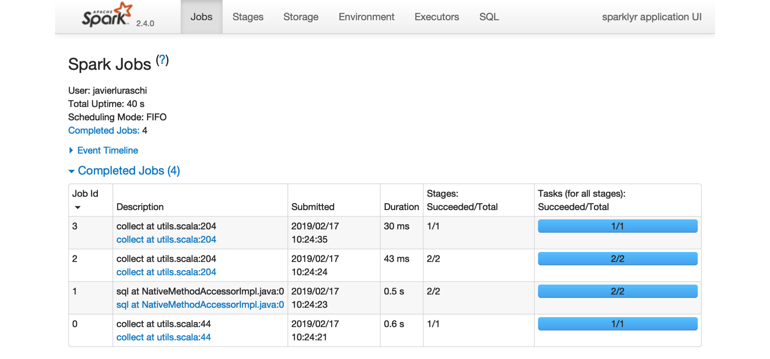
FIGURE 2.1: The Apache Spark web interface
Printing the cars dataset collected a few records to be displayed in the R console. You can see in the Spark web interface that a job was started to collect this information back from Spark. You can also select the Storage tab to see the mtcars dataset cached in memory in Spark, as shown in Figure 2.2.
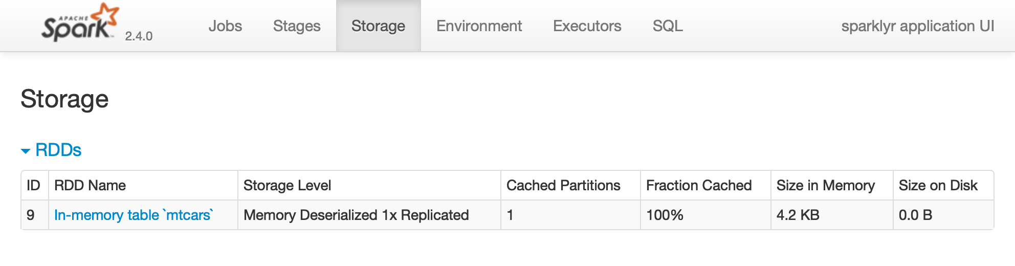
FIGURE 2.2: The Storage tab on the Apache Spark web interface
Notice that this dataset is fully loaded into memory, as indicated by the Fraction Cached column, which shows 100%; thus, you can see exactly how much memory this dataset is using through the Size in Memory column.
The Executors tab, shown in Figure 2.3, provides a view of your cluster resources. For local connections, you will find only one executor active with only 2 GB of memory allocated to Spark, and 384 MB available for computation. In Chapter 9 you will learn how to request more compute instances and resources, and how memory is allocated.
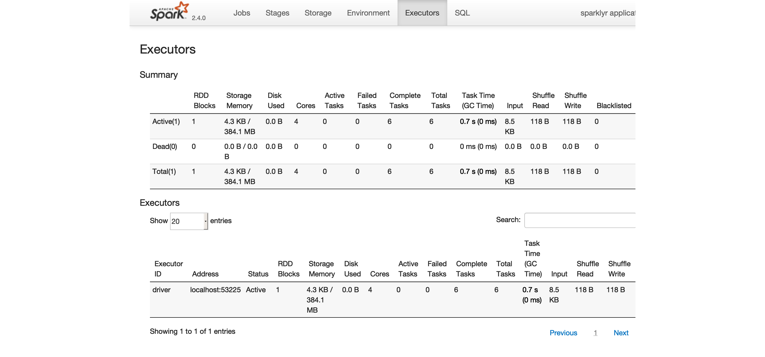
FIGURE 2.3: The Executors tab on the Apache Spark web interface
The last tab to explore is the Environment tab, shown in Figure 2.4; this tab lists all of the settings for this Spark application, which we look at in Chapter 9. As you will learn, most settings don’t need to be configured explicitly, but to properly run them at scale, you need to become familiar with some of them, eventually.
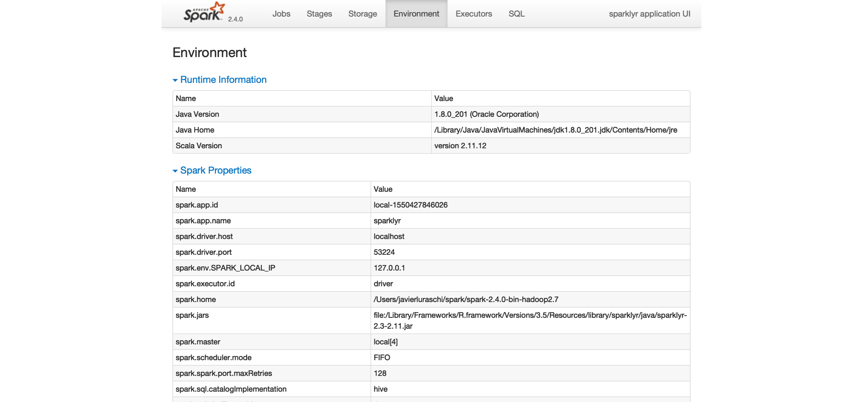
FIGURE 2.4: The Environment tab on the Apache Spark web interface
Next, you will make use of a small subset of the practices that we cover in depth in Chapter 3.
2.4.2 Analysis
When using Spark from R to analyze data, you can use SQL (Structured Query Language) or dplyr (a grammar of data manipulation). You can use SQL through the DBI package; for instance, to count how many records are available in our cars dataset, we can run the following:
  count(1)
1       32
When using dplyr, you write less code, and it’s often much easier to write than SQL. This is precisely why we won’t make use of SQL in this book; however, if you are proficient in SQL, this is a viable option for you. For instance, counting records in dplyr is more compact and easier to understand:
# Source: spark<?> [?? x 1]
      n
  <dbl>
1    32
In general, we usually start by analyzing data in Spark with dplyr, followed by sampling rows and selecting a subset of the available columns. The last step is to collect data from Spark to perform further data processing in R, like data visualization. Let’s perform a very simple data analysis example by selecting, sampling, and plotting the cars dataset in Spark:
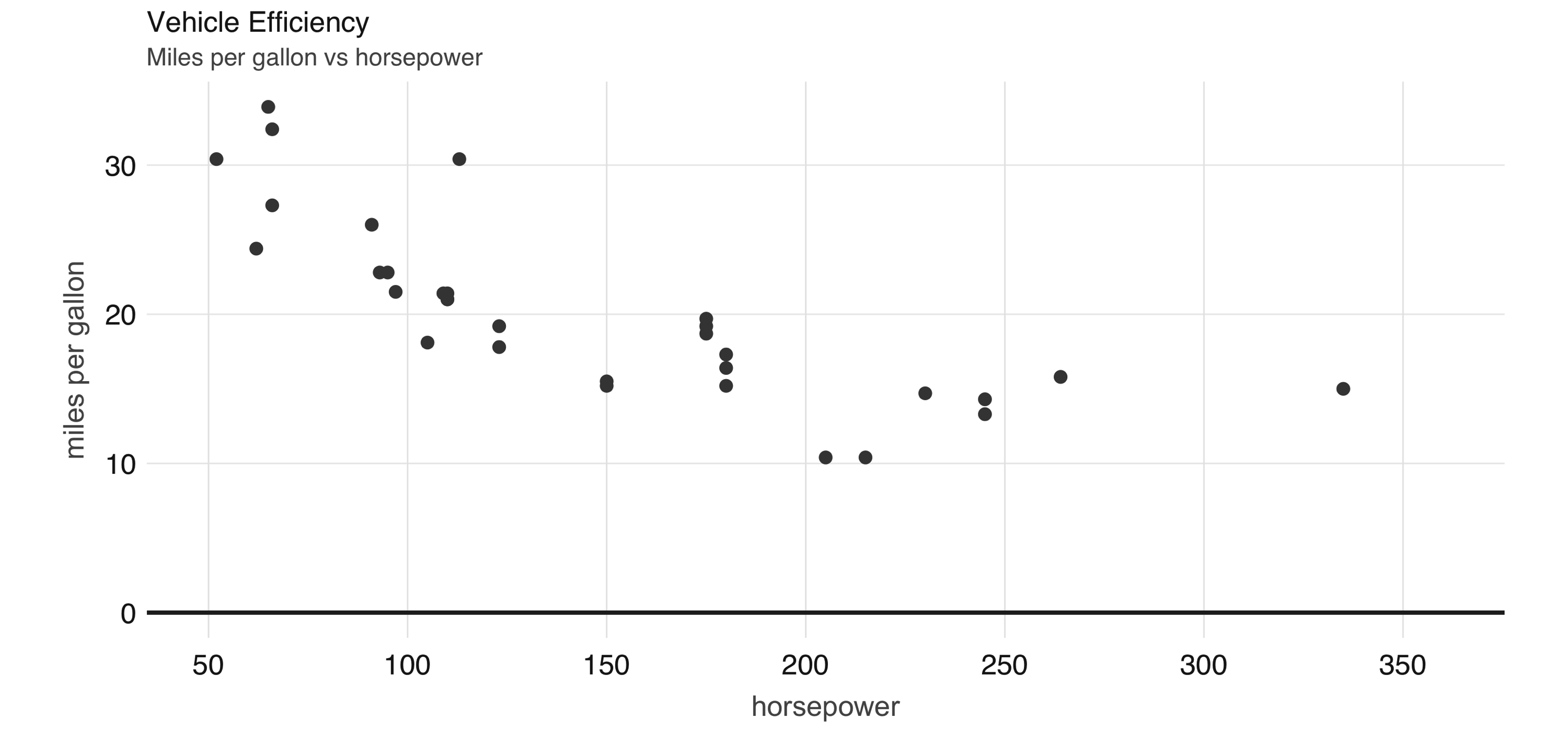
FIGURE 2.5: Horsepower versus miles per gallon
The plot in Figure 2.5, shows that as we increase the horsepower in a vehicle, its fuel efficiency measured in miles per gallon decreases. Although this is insightful, it’s difficult to predict numerically how increased horsepower would affect fuel efficiency. Modeling can help us overcome this.
2.4.3 Modeling
Although data analysis can take you quite far toward understanding data, building a mathematical model that describes and generalizes the dataset is quite powerful. In Chapter 1 you learned that the fields of machine learning and data science make use of mathematical models to perform predictions and find additional insights.
For instance, we can use a linear model to approximate the relationship between fuel efficiency and horsepower:
Formula: mpg ~ hp

Coefficients:
(Intercept)          hp
30.09886054 -0.06822828
Now we can use this model to predict values that are not in the original dataset. For instance, we can add entries for cars with horsepower beyond 250 and also visualize the predicted values, as shown in Figure 2.6.
model %>%
  ml_predict(copy_to(sc, data.frame(hp = 250 + 10 * 1:10))) %>%
  transmute(hp = hp, mpg = prediction) %>%
  full_join(select(cars, hp, mpg)) %>%
  collect() %>%
  plot()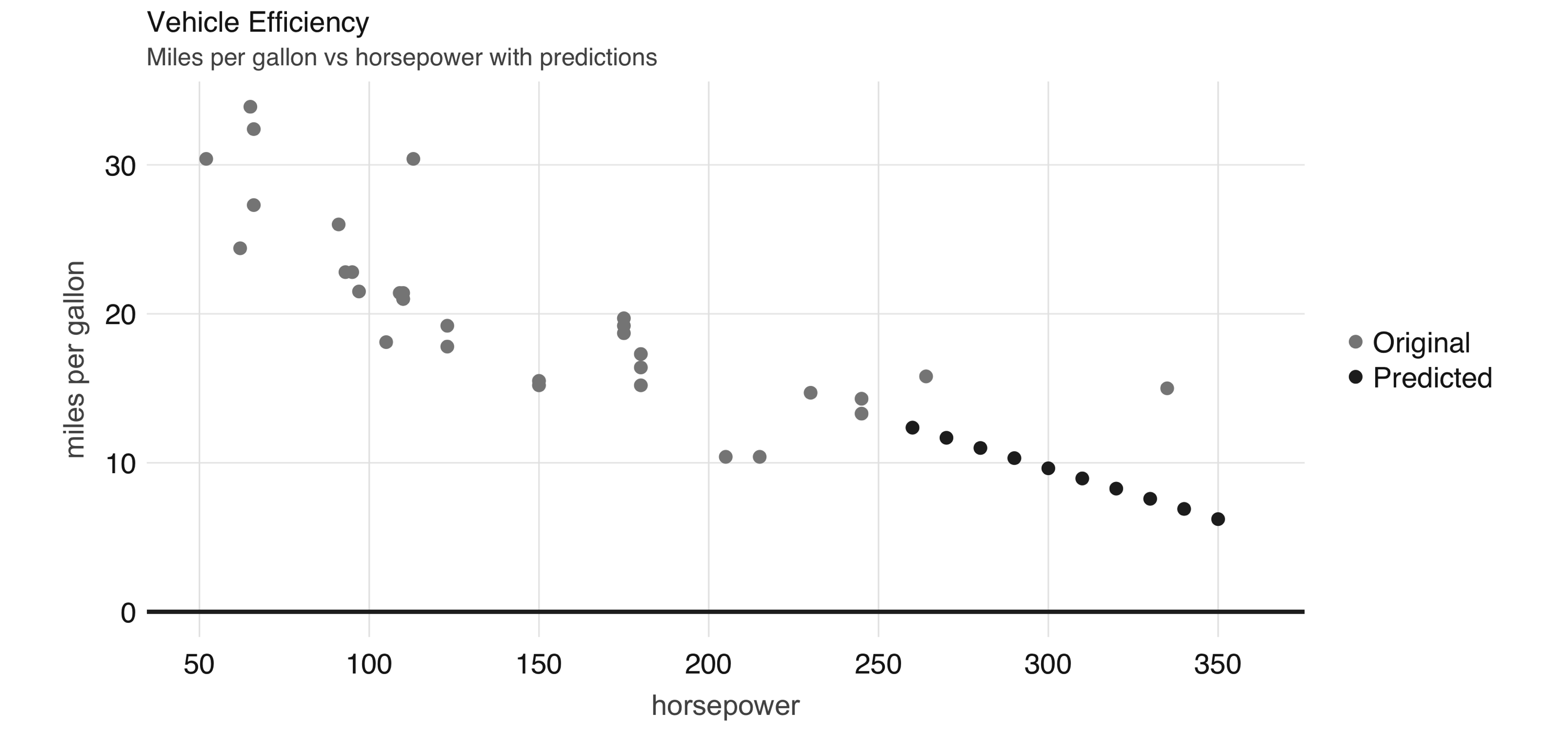
FIGURE 2.6: Horsepower versus miles per gallon with predictions
Even though the previous example lacks many of the appropriate techniques that you should use while modeling, it’s also a simple example to briefly introduce the modeling capabilities of Spark. We introduce all of the Spark models, techniques, and best practices in Chapter 4.
2.4.4 Data
For simplicity, we copied the mtcars dataset into Spark; however, data is usually not copied into Spark. Instead, data is read from existing data sources in a variety of formats, like plain text, CSV, JSON, Java Database Connectivity (JDBC), and many more, which we examine in detail in Chapter 8. For instance, we can export our cars dataset as a CSV file:
In practice, we would read an existing dataset from a distributed storage system like HDFS, but we can also read back from the local file system:
2.4.5 Extensions
In the same way that R is known for its vibrant community of package authors, at a smaller scale, many extensions for Spark and R have been written and are available to you. Chapter 10 introduces many interesting ones to perform advanced modeling, graph analysis, preprocessing of datasets for deep learning, and more.
For instance, the sparkly.nested extension is an R package that extends sparklyr to help you manage values that contain nested information. A common use case involves JSON files that contain nested lists that require preprocessing before you can do meaningful data analysis. To use this extension, we first need to install it as follows:
Then, we can use the sparklyr.nested extension to group all of the horsepower data points over the number of cylinders:
# Source: spark<?> [?? x 2]
    cyl data
  <int> <list>
1     6 <list [7]>
2     4 <list [11]>
3     8 <list [14]>
Even though nesting data makes it more difficult to read, it is a requirement when you are dealing with nested data formats like JSON using the spark_read_json() and spark_write_json() functions.
2.4.6 Distributed R
For those few cases when a particular functionality is not available in Spark and no extension has been developed, you can consider distributing your own R code across the Spark cluster. This is a powerful tool, but it comes with additional complexity, so you should only use it as a last resort.
Suppose that we need to round all of the values across all the columns in our dataset. One approach would be running custom R code, making use of R’s round() function:
# Source: spark<?> [?? x 11]
     mpg   cyl  disp    hp  drat    wt  qsec    vs    am  gear  carb
   <dbl> <dbl> <dbl> <dbl> <dbl> <dbl> <dbl> <dbl> <dbl> <dbl> <dbl>
 1    21     6   160   110     4     3    16     0     1     4     4
 2    21     6   160   110     4     3    17     0     1     4     4
 3    23     4   108    93     4     2    19     1     1     4     1
 4    21     6   258   110     3     3    19     1     0     3     1
 5    19     8   360   175     3     3    17     0     0     3     2
 6    18     6   225   105     3     3    20     1     0     3     1
 7    14     8   360   245     3     4    16     0     0     3     4
 8    24     4   147    62     4     3    20     1     0     4     2
 9    23     4   141    95     4     3    23     1     0     4     2
10    19     6   168   123     4     3    18     1     0     4     4
# … with more rows
If you are a proficient R user, it can be quite tempting to use spark_apply() for everything, but please, don’t! spark_apply() was designed for advanced use cases where Spark falls short. You will learn how to do proper data analysis and modeling without having to distribute custom R code across your cluster.
2.4.7 Streaming
While processing large static datasets is the most typical use case for Spark, processing dynamic datasets in real time is also possible and, for some applications, a requirement. You can think of a streaming dataset as a static data source with new data arriving continuously, like stock market quotes. Streaming data is usually read from Kafka (an open source stream-processing software platform) or from distributed storage that receives new data continuously.
To try out streaming, let’s first create an input/ folder with some data that we will use as the input for this stream:
Then, we define a stream that processes incoming data from the input/ folder, performs a custom transformation in R, and pushes the output into an output/ folder:
As soon as the stream of real-time data starts, the input/ folder is processed and turned into a set of new files under the output/ folder containing the new transformed files. Since the input contained only one file, the output folder will also contain a single file resulting from applying the custom spark_apply() transformation.
[1] "part-00000-eece04d8-7cfa-4231-b61e-f1aef8edeb97-c000.csv"Up to this point, this resembles static data processing; however, we can keep adding files to the input/ location, and Spark will parallelize and process data automatically. Let’s add one more file and validate that it’s automatically processed:
Wait a few seconds and validate that the data is processed by the Spark stream:
[1] "part-00000-2d8e5c07-a2eb-449d-a535-8a19c671477d-c000.csv"
[2] "part-00000-eece04d8-7cfa-4231-b61e-f1aef8edeb97-c000.csv"
You should then stop the stream:
You can use dplyr, SQL, Spark models, or distributed R to analyze streams in real time. In Chapter 12 we properly introduce you to all the interesting transformations you can perform to analyze real-time data.
2.4.8 Logs
Logging is definitely less interesting than real-time data processing; however, it’s a tool you should be or become familiar with. A log is just a text file to which Spark appends information relevant to the execution of tasks in the cluster. For local clusters, we can retrieve all the recent logs by running the following:
18/10/09 19:41:46 INFO Executor: Finished task 0.0 in stage 5.0 (TID 5)...
18/10/09 19:41:46 INFO TaskSetManager: Finished task 0.0 in stage 5.0...
18/10/09 19:41:46 INFO TaskSchedulerImpl: Removed TaskSet 5.0, whose...
18/10/09 19:41:46 INFO DAGScheduler: ResultStage 5 (collect at utils...
18/10/09 19:41:46 INFO DAGScheduler: Job 3 finished: collect at utils...
Or, we can retrieve specific log entries containing, say, sparklyr, by using the filter parameter, as follows:
## 18/10/09 18:53:23 INFO SparkContext: Submitted application: sparklyr
## 18/10/09 18:53:23 INFO SparkContext: Added JAR...
## 18/10/09 18:53:27 INFO Executor: Fetching spark://localhost:52930/...
## 18/10/09 18:53:27 INFO Utils: Fetching spark://localhost:52930/...
## 18/10/09 18:53:27 INFO Executor: Adding file:/private/var/folders/...
Most of the time, you won’t need to worry about Spark logs, except in cases for which you need to troubleshoot a failed computation; in those cases, logs are an invaluable resource to be aware of. Now you know.
2.5 Disconnecting
For local clusters (really, any cluster), after you are done processing data, you should disconnect by running the following:
This terminates the connection to the cluster as well as the cluster tasks. If multiple Spark connections are active, or if the connection instance sc is no longer available, you can also disconnect all your Spark connections by running this command:
Notice that exiting R, or RStudio, or restarting your R session, also causes the Spark connection to terminate, which in turn terminates the Spark cluster and cached data that is not explicitly saved.
2.6 Using RStudio
Since it’s very common to use RStudio with R, sparklyr provides RStudio extensions to help simplify your workflows and increase your productivity while using Spark in RStudio. If you are not familiar with RStudio, take a quick look at Using RStudio. Otherwise, there are a couple extensions worth highlighting.
First, instead of starting a new connection using spark_connect() from RStudio’s R console, you can use the New Connection action from the Connections tab and then select the Spark connection, which opens the dialog shown in Figure 2.7. You can then customize the versions and connect to Spark, which will simply generate the right spark_connect() command and execute this in the R console for you.
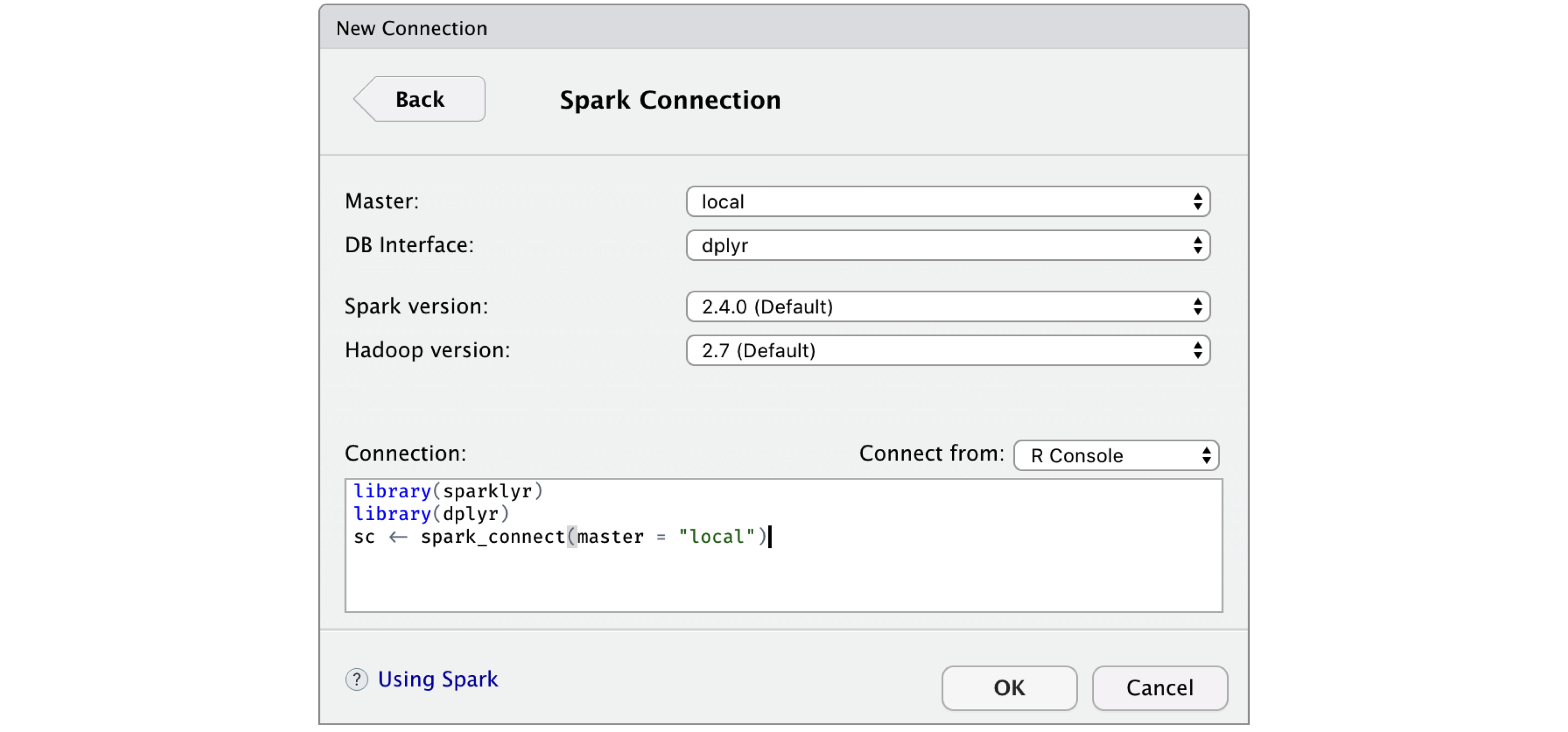
FIGURE 2.7: RStudio New Spark Connection dialog
After you’re connected to Spark, RStudio displays your available datasets in the Connections tab, as shown in Figure 2.8. This is a useful way to track your existing datasets and provides an easy way to explore each of them.
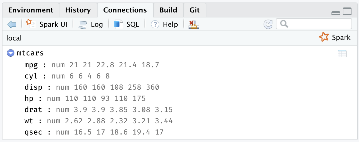
FIGURE 2.8: The RStudio Connections tab
Additionally, an active connection provides the following custom actions:
- Spark
- Opens the Spark web interface; a shortcut to
spark_web(sc). - Log
- Opens the Spark web logs; a shortcut to
spark_log(sc). - SQL
- Opens a new SQL query. For more information about
DBIand SQL support, see Chapter 3. - Help
- Opens the reference documentation in a new web browser window.
- Disconnect
- Disconnects from Spark; a shortcut to
spark_disconnect(sc).
The rest of this book will use plain R code. It is up to you whether to execute this code in the R console, RStudio, Jupyter Notebooks, or any other tool that supports executing R code, since the examples provided in this book execute in any R environment.
2.7 Resources
While we’ve put significant effort into simplifying the onboarding process, there are many additional resources that can help you to troubleshoot particular issues while getting started and, in general, introduce you to the broader Spark and R communities to help you get specific answers, discuss topics, and connect with many users actively using Spark with R:
- Documentation
- The documentation site hosted in RStudio’s Spark website should be your first stop to learn more about Spark when using R. The documentation is kept up to date with examples, reference functions, and many more relevant resources.
- Blog
- To keep up to date with major
sparklyrannouncements, you can follow the RStudio blog. - Community
- For general
sparklyrquestions, you can post in the RStudio Community tagged assparklyr. - Stack Overflow
- For general Spark questions, Stack Overflow is a great resource; there are also many topics specifically about
sparklyr. - Github
- If you believe something needs to be fixed, open a GitHub issue or send us a pull request.
- Gitter
- For urgent issues or to keep in touch, you can chat with us in Gitter.
2.8 Recap
In this chapter you learned about the prerequisites required to work with Spark. You saw how to connect to Spark using spark_connect(); install a local cluster using spark_install(); load a simple dataset, launch the web interface, and display logs using spark_web(sc) and spark_log(sc), respectively; and disconnect from RStudio using spark_disconnect(). We close by presenting the RStudio extensions that sparklyr provides.
At this point, we hope that you feel ready to tackle actual data analysis and modeling problems in Spark and R, which will be introduced over the next two chapters. Chapter 3 will present data analysis as the process of inspecting, cleaning, and transforming data with the goal of discovering useful information. Modeling, the subject of Chapter 4, can be considered part of data analysis; however, it deserves its own chapter to truly describe and take advantage of the modeling functionality available in Spark.