Chapter 10 Extensions
I try to know as many people as I can. You never know which one you’ll need.
— Tyrion Lannister
In Chapter 9, you learned how Spark processes data at large scale by allowing users to configure the cluster resources, partition data implicitly or explicitly, execute commands across distributed compute nodes, shuffle data across them when needed, cache data to improve performance, and serialize data efficiently over the network. You also learned how to configure the different Spark settings used while connecting, submitting a job, and running an application, as well as particular settings applicable only to R and R extensions that we present in this chapter.
Chapters 3-4, and 8 provided a foundation to read and understand most datasets. However, the functionality that was presented was scoped to Spark’s built-in features and tabular datasets. This chapter goes beyond tabular data and explores how to analyze and model networks of interconnected objects through graph processing, analyze genomics datasets, prepare data for deep learning, analyze geographic datasets, and use advanced modeling libraries like H2O and XGBoost over large-scale datasets.
The combination of all the content presented in the previous chapters should take care of most of your large-scale computing needs. However, for those few use cases for which functionality is still lacking, the following chapters provide tools to extend Spark yourself—through custom R transformation, custom Scala code, or a recent new execution mode in Spark that enables analyzing real-time datasets. However, before reinventing the wheel, let’s examine some of the extensions available in Spark.
10.1 Overview
In Chapter 1, we presented the R community as a vibrant group of individuals collaborating with each other in many ways—for example, moving open science forward by creating R packages that you can install from CRAN. In a similar way, but at a much smaller scale, the R community has contributed extensions that increase the functionality initially supported in Spark and R. Spark itself also provides support for creating Spark extensions and, in fact, many R extensions make use of Spark extensions.
Extensions are constantly being created, so this section will be outdated at some given point in time. In addition, we might not even be aware of many Spark and R extensions. However, at the very least we can track the extensions that are available in CRAN by looking at the “reverse imports” for sparklyr in CRAN. Extensions and R packages published in CRAN tend to be the most stable since when a package is published in CRAN, it goes through a review process that increases the overall quality of a contribution.
While we wish we could present all the extensions, we’ve instead scoped this chapter to the extensions that should be the most interesting to you. You can find additional extensions at the github.com/r-spark organization or by searching repositories on GitHub with the sparklyr tag.
- rsparkling
- The
rsparklingextensions allows you to use H2O and Spark from R. This extension is what we would consider advanced modeling in Spark. While Spark’s built-in modeling library, Spark MLlib, is quite useful in many cases; H2O’s modeling capabilities can compute additional statistical metrics and can provide performance and scalability improvements over Spark MLlib. We, ourselves, have not performed detailed comparisons nor benchmarks between MLlib and H2O; so this is something you will have to research on your own to create a complete picture of when to use H2O’s capabilities. - graphframes
- The
graphframesextensions adds support to process graphs in Spark. A graph is a structure that describes a set of objects in which some pairs of the objects are in some sense related. As you learned in Chapter 1, ranking web pages was an early motivation to develop precursors to Spark powered by MapReduce; web pages happen to form a graph if you consider a link between pages as the relationship between each pair of pages. Computing operations likes PageRank over graphs can be quite useful in web search and social networks, for example. - sparktf
- The
sparktfextension provides support to write TensorFlow records in Spark. TensorFlow is one of the leading deep learning frameworks, and it is often used with large amounts of numerical data represented as TensorFlow records, a file format optimized for TensorFlow. Spark is often used to process unstructured and large-scale datasets into smaller numerical datasets that can easily fit into a GPU. You can use this extension to save datasets in the TensorFlow record file format. - xgboost
- The
xgboostextension brings the well-known XGBoost modeling library to the world of large-scale computing. XGBoost is a scalable, portable, and distributed library for gradient boosting. It became well known in the machine learning competition circles after its use in the winning solution of the Higgs Boson Machine Learning Challenge and has remained popular in other Kaggle competitions since then. - variantspark
- The
variantsparkextension provides an interface to use Variant Spark, a scalable toolkit for genome-wide association studies (GWAS). It currently provides functionality to build random forest models, estimating variable importance, and reading variant call format (VCF) files. While there are other random forest implementations in Spark, most of them are not optimized to deal with GWAS datasets, which usually come with thousands of samples and millions of pass:[variables]. - geospark
- The
geosparkextension enables us to load and query large-scale geographic datasets. Usually datasets containing latitude and longitude points or complex areas are defined in the well-known text (WKT) format, a text markup language for representing vector geometry objects on a map.
Before you learn how and when to use each extension, we should first briefly explain how you can use extensions with R and Spark.
First, a Spark extension is just an R package that happens to be aware of Spark. As with any other R package, you will first need to install the extension. After you’ve installed it, it is important to know that you will need to reconnect to Spark before the extension can be used. So, in general, here’s the pattern you should follow:
Notice that sparklyr is loaded after the extension to allow the extension to register properly. If you had to install and load a new extension, you would first need to disconnect using spark_disconnect(sc), restart your R session, and repeat the preceding steps with the new extension.
It’s not difficult to install and use Spark extensions from R; however, each extension can be a world of its own, so most of the time you will need to spend time understanding what the extension is, when to use it, and how to use it properly. The first extension you will learn about is the rsparkling extension, which enables you to use H2O in Spark with R.
10.2 H2O
H2O, created by H2O.ai, is open source software for large-scale modeling that allows you to fit thousands of potential models as part of discovering patterns in data. You can consider using H2O to complement or replace Spark’s default modeling algorithms. It is common to use Spark’s default modeling algorithms and transition to H2O when Spark’s algorithms fall short or when advanced functionality (like additional modeling metrics or automatic model selection) is desired.
We can’t do justice to H2O’s great modeling capabilities in a single paragraph; explaining H2O properly would require a book in and of itself. Instead, we would like to recommend reading Darren Cook’s Practical Machine Learning with H2O (O’Reilly) to explore in-depth H2O’s modeling algorithms and features. In the meantime, you can use this section as a brief guide to get started using H2O in Spark with R.
To use H2O with Spark, it is important to know that there are four components involved: H2O, Sparkling Water, rsparkling, and Spark. Sparkling Water allows users to combine the fast, scalable machine learning algorithms of H2O with the capabilities of Spark. You can think of Sparkling Water as a component bridging Spark with H2O and rsparkling as the R frontend for Sparkling Water, as depicted in Figure 10.1.
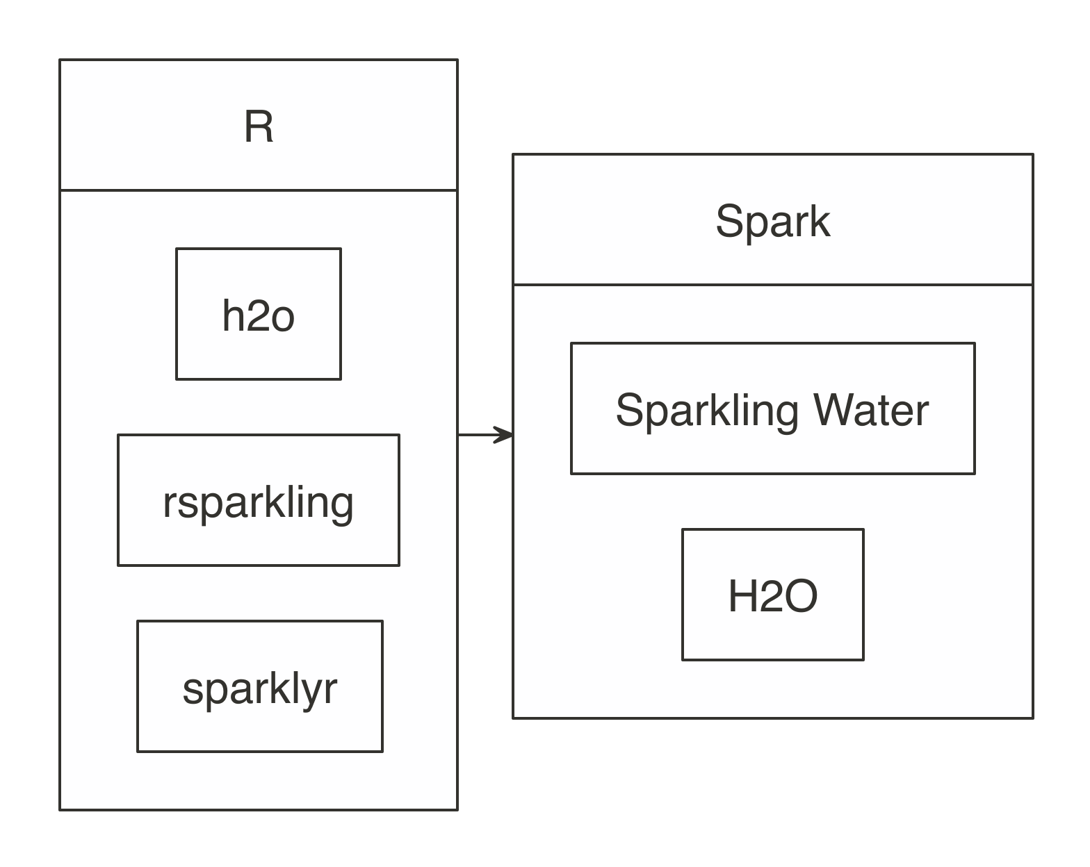
FIGURE 10.1: H2O components with Spark and R
First, install rsparkling and h2o as specified on the rsparkling documentation site.
install.packages("h2o", type = "source",
  repos = "http://h2o-release.s3.amazonaws.com/h2o/rel-yates/5/R")
install.packages("rsparkling", type = "source",
  repos = "http://h2o-release.s3.amazonaws.com/sparkling-water/rel-2.3/31/R")
It is important to note that you need to use compatible versions of Spark, Sparkling Water, and H2O as specified in their documentation; we present instructions for Spark 2.3, but using different Spark versions will require you to install different versions. So let’s start by checking the version of H2O by running the following:
## [1] '3.26.0.2'## [1] '0.2.18'We then can connect with the supported Spark versions as follows (you will have to adjust the master parameter for your particular cluster):
library(rsparkling)
library(sparklyr)
library(h2o)

sc <- spark_connect(master = "local", version = "2.3",
                    config = list(sparklyr.connect.timeout = 3 * 60))

cars <- copy_to(sc, mtcars)
H2O provides a web interface that can help you monitor training and access much of H2O’s functionality. You can access the web interface (called H2O Flow) through h2o_flow(sc), as shown in Figure 10.2.
When using H2O, you will have to convert your Spark DataFrame into and H2O DataFrame through as_h2o_frame:
   mpg cyl disp  hp drat    wt  qsec vs am gear carb
1 21.0   6  160 110 3.90 2.620 16.46  0  1    4    4
2 21.0   6  160 110 3.90 2.875 17.02  0  1    4    4
3 22.8   4  108  93 3.85 2.320 18.61  1  1    4    1
4 21.4   6  258 110 3.08 3.215 19.44  1  0    3    1
5 18.7   8  360 175 3.15 3.440 17.02  0  0    3    2
6 18.1   6  225 105 2.76 3.460 20.22  1  0    3    1

[32 rows x 11 columns] 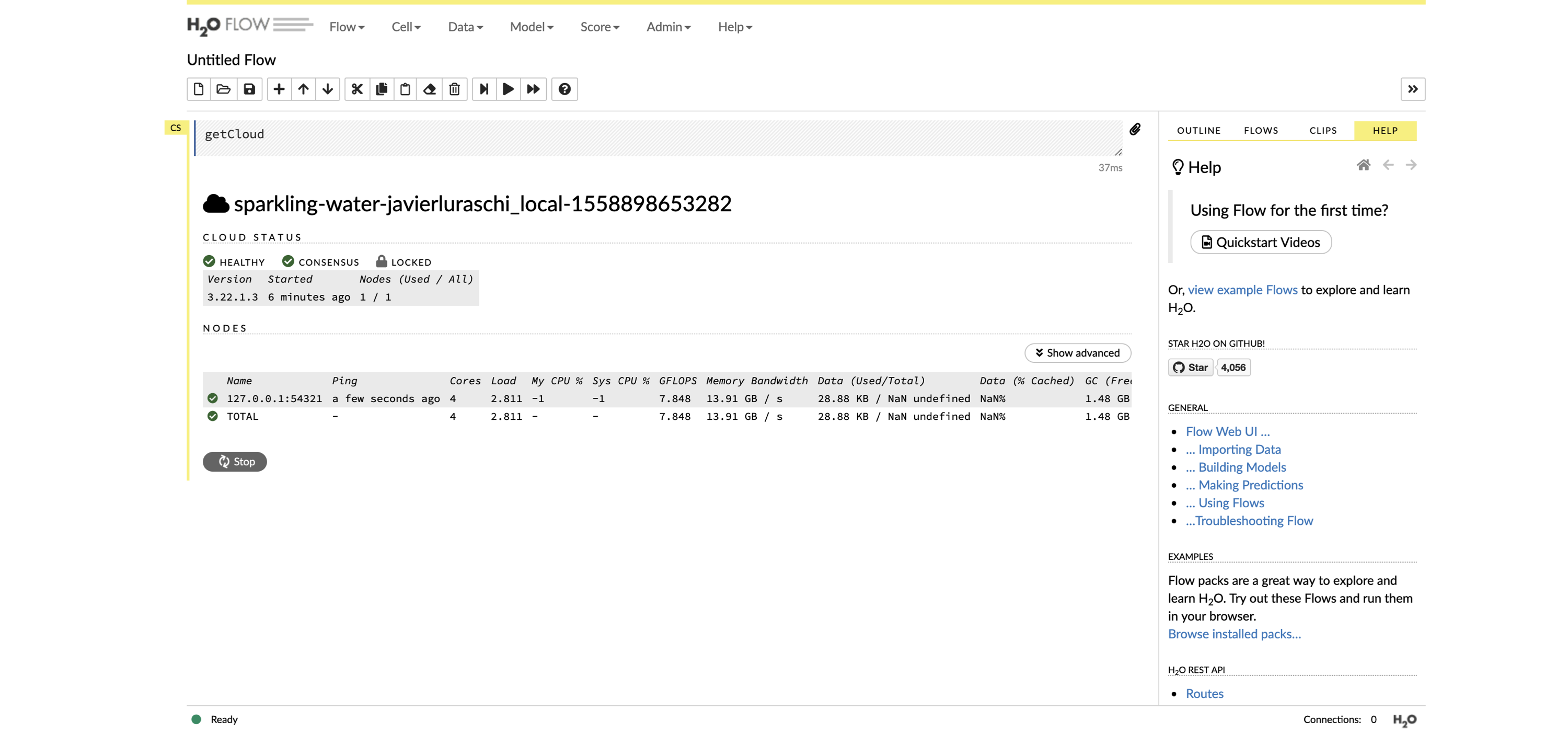
FIGURE 10.2: The H2O Flow interface using Spark with R
Then, you can use many of the modeling functions available in the h2o package with ease. For instance, we can fit a generalized linear model with ease:
H2O provides additional metrics not necessarily available in Spark’s modeling algorithms. The model that we just fit, Residual Deviance, is provided in the model, while this would not be a standard metric when using Spark MLlib.
...
MSE:  6.017684
RMSE:  2.453097
MAE:  1.940985
RMSLE:  0.1114801
Mean Residual Deviance :  6.017684
R^2 :  0.8289895
Null Deviance :1126.047
Null D.o.F. :31
Residual Deviance :192.5659
Residual D.o.F. :29
AIC :156.2425
Then, you can run prediction over the generalized linear model (GLM). A similar approach would work for many other models available in H2O:
predictions <- as_h2o_frame(sc, copy_to(sc, data.frame(wt = 2, cyl = 6)))
h2o.predict(model, predictions)
predict
1 24.05984
[1 row x 1 column]You can also use H2O to perform automatic training and tuning of many models, meaning that H2O can choose which model to use for you using AutoML:
automl <- h2o.automl(x = c("wt", "cyl"), y = "mpg",
                     training_frame = cars_h2o,
                     max_models = 20,
                     seed = 1)
For this particular dataset, H2O determines that a deep learning model is a better fit than a GLM.22 Specifically, H2O’s AutoML explored using XGBoost, deep learning, GLM, and a Stacked Ensemble model:
model_id              mean_residual_dev…     rmse      mse      mae     rmsle
1 DeepLearning_…                6.541322 2.557601 6.541322 2.192295 0.1242028
2 XGBoost_grid_1…               6.958945 2.637981 6.958945 2.129421 0.1347795
3 XGBoost_grid_1_…              6.969577 2.639996 6.969577 2.178845 0.1336290
4 XGBoost_grid_1_…              7.266691 2.695680 7.266691 2.167930 0.1331849
5 StackedEnsemble…              7.304556 2.702694 7.304556 1.938982 0.1304792
6 XGBoost_3_…                   7.313948 2.704431 7.313948 2.088791 0.1348819
Rather than using the leaderboard, you can focus on the best model through automl@leader; for example, you can glance at the particular parameters from this deep learning model as follows:
tibble::tibble(parameter = names(automl@leader@parameters),
               value = as.character(automl@leader@parameters))
# A tibble: 20 x 2
parameter values
<chr> <chr>
1 model_id DeepLearning_grid_1_AutoML…
2 training_frame automl_training_frame_rdd…
3 nfolds 5
4 keep_cross_validation_models FALSE
5 keep_cross_validation_predictions TRUE
6 fold_assignment Modulo
7 overwrite_with_best_model FALSE
8 activation RectifierWithDropout
9 hidden 200
10 epochs 10003.6618461538
11 seed 1
12 rho 0.95
13 epsilon 1e-06
14 input_dropout_ratio 0.2
15 hidden_dropout_ratios 0.4
16 stopping_rounds 0
17 stopping_metric deviance
18 stopping_tolerance 0.05
19 x c("cyl", "wt")
20 y mpg You can then predict using the leader as follows:
   predict
1 30.74639

[1 row x 1 column]
Many additional examples are available, and you can also request help from the official GitHub repository for the rsparkling package.
The next extension, graphframes, allows you to process large-scale relational datasets. Before you start using it, make sure to disconnect with spark_disconnect(sc) and restart your R session since using a different extension requires you to reconnect to Spark and reload sparklyr.
10.3 Graphs
The first paper in the history of graph theory was written by Leonhard Euler on the Seven Bridges of Königsberg in 1736. The problem was to devise a walk through the city that would cross each bridge once and only once. Figure 10.3 presents the original diagram.

FIGURE 10.3: The Seven Bridges of Königsberg from the Euler archive
Today, a graph is defined as an ordered pair \(G=(V,E)\), with \(V\) a set of vertices (nodes or points) and \(E \subseteq \{\{x, y\} | (x, y) ∈ \mathrm{V}^2 \land x \ne y\}\) a set of edges (links or lines), which are either an unordered pair for undirected graphs or an ordered pair for directed graphs. The former describes links where the direction does not matter, and the latter describes links where it does.
As a simple example, we can use the highschool dataset from the ggraph package, which tracks friendship among high school boys. In this dataset, the vertices are the students and the edges describe pairs of students who happen to be friends in a particular year:
# A tibble: 506 x 3
    from    to  year
   <dbl> <dbl> <dbl>
 1     1    14  1957
 2     1    15  1957
 3     1    21  1957
 4     1    54  1957
 5     1    55  1957
 6     2    21  1957
 7     2    22  1957
 8     3     9  1957
 9     3    15  1957
10     4     5  1957
# … with 496 more rows
While the high school dataset can easily be processed in R, even medium-size graph datasets can be difficult to process without distributing this work across a cluster of machines, for which Spark is well suited. Spark supports processing graphs through the graphframes extension, which in turn uses the GraphX Spark component. GraphX is Apache Spark’s API for graphs and graph-parallel computation. It’s comparable in performance to the fastest specialized graph-processing systems and provides a growing library of graph algorithms.
A graph in Spark is also represented as a DataFrame of edges and vertices; however, our format is slightly different since we will need to construct a DataFrame for vertices. Let’s first install the graphframes extension:
Next, we need to connect, copying the highschool dataset and transforming the graph to the format that this extension expects. Here, we scope this dataset to the friendships of the year 1957:
library(graphframes)
library(sparklyr)
library(dplyr)

sc <- spark_connect(master = "local", version = "2.3")
highschool_tbl <- copy_to(sc, ggraph::highschool, "highschool") %>%
  filter(year == 1957) %>%
  transmute(from = as.character(as.integer(from)),
            to = as.character(as.integer(to)))

from_tbl <- highschool_tbl %>% distinct(from) %>% transmute(id = from)
to_tbl <- highschool_tbl %>% distinct(to) %>% transmute(id = to)

vertices_tbl <- distinct(sdf_bind_rows(from_tbl, to_tbl))
edges_tbl <- highschool_tbl %>% transmute(src = from, dst = to)
The vertices_tbl table is expected to have a single id column:
# Source: spark<?> [?? x 1]
   id
   <chr>
 1 1
 2 34
 3 37
 4 43
 5 44
 6 45
 7 56
 8 57
 9 65
10 71
# … with more rows
And the edges_tbl is expected to have src and dst columns:
# Source: spark<?> [?? x 2]
   src   dst
   <chr> <chr>
 1 1     14
 2 1     15
 3 1     21
 4 1     54
 5 1     55
 6 2     21
 7 2     22
 8 3     9
 9 3     15
10 4     5
# … with more rows
You can now create a GraphFrame:
We now can use this graph to start analyzing this dataset. For instance, we’ll find out how many friends on average every boy has, which is referred to as the degree or valency of a vertex:
# Source: spark<?> [?? x 1]
  friends
    <dbl>
1    6.94
We then can find what the shortest path to some specific vertex (a boy for this dataset). Since the data is anonymized, we can just pick the boy identified as 33 and find how many degrees of separation exist between them:
gf_shortest_paths(graph, 33) %>%
  filter(size(distances) > 0) %>%
  mutate(distance = explode(map_values(distances))) %>%
  select(id, distance)
# Source: spark<?> [?? x 2]
id distance
<chr> <int>
1 19 5
2 5 4
3 27 6
4 4 4
5 11 6
6 23 4
7 36 1
8 26 2
9 33 0
10 18 5
# … with more rowsFinally, we can also compute PageRank over this graph, which was presented in Chapter 1’s discussion of Google’s page ranking algorithm:
GraphFrame
Vertices:
  Database: spark_connection
  $ id       <dbl> 12, 12, 14, 14, 27, 27, 55, 55, 64, 64, 41, 41, 47, 47, 6…
  $ pagerank <dbl> 0.3573460, 0.3573460, 0.3893665, 0.3893665, 0.2362396, 0.…
Edges:
  Database: spark_connection
  $ src    <dbl> 7, 7, 7, 7, 7, 7, 7, 7, 7, 7, 7, 7, 7, 7, 7, 7, 12, 12, 12,…
  $ dst    <dbl> 17, 17, 17, 17, 17, 17, 17, 17, 17, 17, 17, 17, 17, 17, 17,…
  $ weight <dbl> 0.25000000, 0.25000000, 0.25000000, 0.25000000, 0.25000000,…
To give you some insights into this dataset, Figure 10.4 plots this chart using the ggraph and highlights the highest PageRank scores for the following dataset:
highschool_tbl %>%
  igraph::graph_from_data_frame(directed = FALSE) %>%
  ggraph(layout = 'kk') +
    geom_edge_link(alpha = 0.2,
                   arrow = arrow(length = unit(2, 'mm')),
                   end_cap = circle(2, 'mm'),
                   start_cap = circle(2, 'mm')) +
    geom_node_point(size = 2, alpha = 0.4)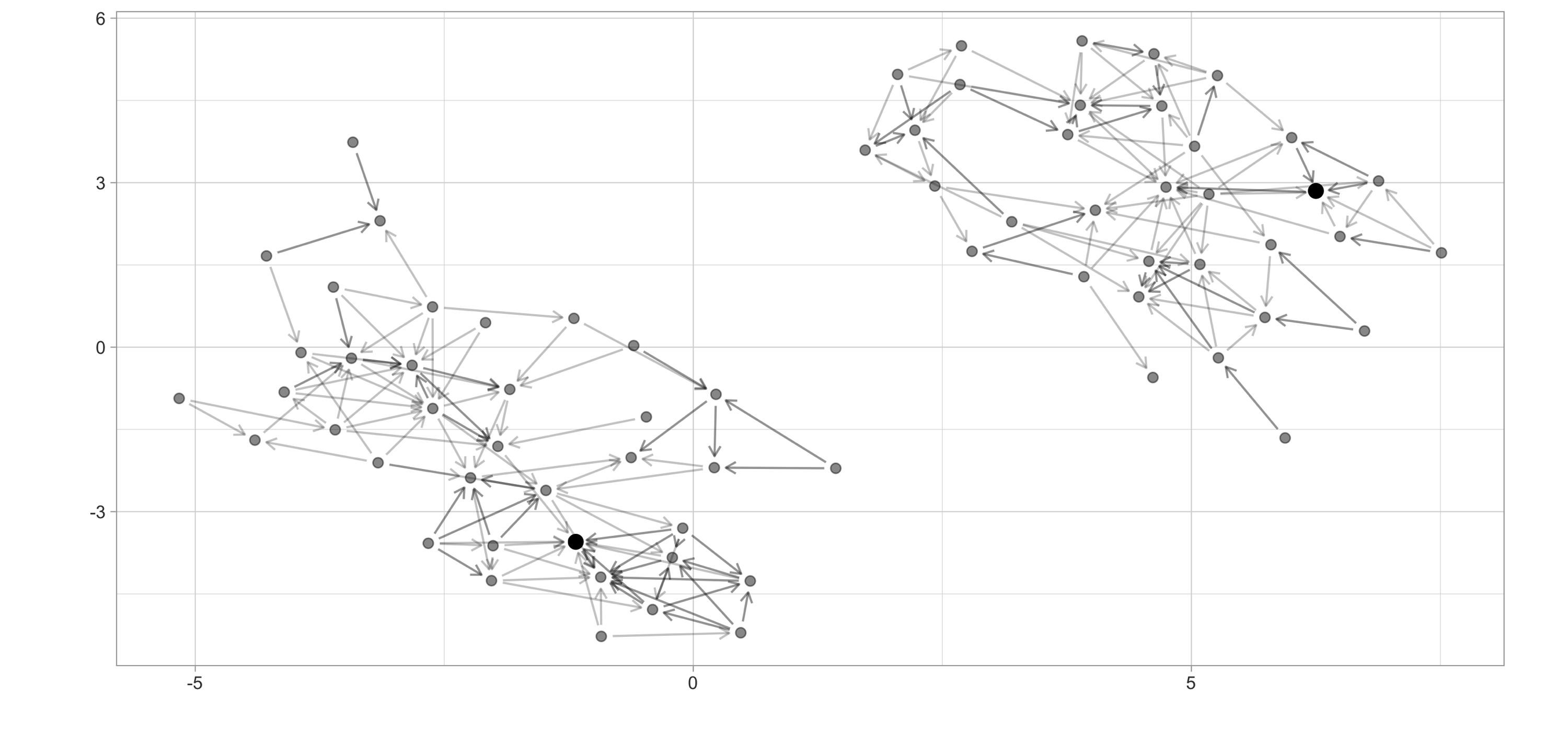
FIGURE 10.4: High school ggraph dataset with highest PageRank highlighted
There are many more graph algorithms provided in graphframes—for example, breadth-first search, connected components, label propagation for detecting communities, strongly connected components, and triangle count. For questions on this extension refer to the official GitHub repository. We now present a popular gradient-boosting framework—make sure to disconnect and restart before trying the next extension.
10.4 XGBoost
A decision tree is a flowchart-like structure in which each internal node represents a test on an attribute, each branch represents the outcome of the test, and each leaf node represents a class label. For example, Figure 10.5 shows a decision tree that could help classify whether an employee is likely to leave given a set of factors like job satisfaction and overtime. When a decision tree is used to predict continuous variables instead of discrete outcomes—say, how likely someone is to leave a company—it is referred to as a regression tree.
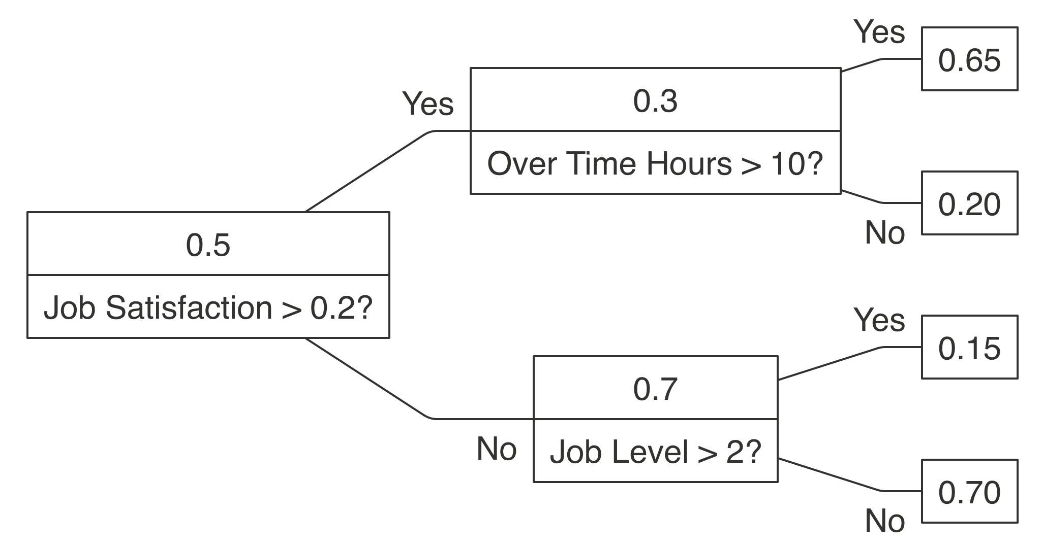
FIGURE 10.5: A decision tree to predict job attrition based on known factors
While a decision tree representation is quite easy to understand and to interpret, finding out the decisions in the tree requires mathematical techniques like gradient descent to find a local minimum. Gradient descent takes steps proportional to the negative of the gradient of the function at the current point. The gradient is represented by \(\nabla\), and the learning rate by \(\gamma\). You simply start from a given state \(a_n\) and compute the next iteration \(a_{n+1}\) by following the direction of the gradient:
XGBoost is an open source software library that provides a gradient-boosting framework. It aims to provide scalable, portable, and distributed gradient boosting for training gradient-boosted decision trees (GBDT) and gradient-boosted regression trees (GBRT). Gradient-boosted means XGBoost uses gradient descent and boosting, which is a technique that chooses each predictor sequentially.
sparkxgb is an extension that you can use to train XGBoost models in Spark; however, be aware that currently Windows is unsupported. To use this extension, first install it from CRAN:
Then, you need to import the sparkxgb extension followed by your usual Spark connection code, adjusting master as needed:
library(sparkxgb)
library(sparklyr)
library(dplyr)

sc <- spark_connect(master = "local", version = "2.3")
For this example, we use the attrition dataset from the rsample package, which you would need to install by using install.packages("rsample"). This is a fictional dataset created by IBM data scientists to uncover the factors that lead to employee attrition:
# Source: spark<?> [?? x 31]
     Age Attrition BusinessTravel DailyRate Department DistanceFromHome
   <int> <chr>     <chr>              <int> <chr>                 <int>
 1    41 Yes       Travel_Rarely       1102 Sales                     1
 2    49 No        Travel_Freque…       279 Research_…                8
 3    37 Yes       Travel_Rarely       1373 Research_…                2
 4    33 No        Travel_Freque…      1392 Research_…                3
 5    27 No        Travel_Rarely        591 Research_…                2
 6    32 No        Travel_Freque…      1005 Research_…                2
 7    59 No        Travel_Rarely       1324 Research_…                3
 8    30 No        Travel_Rarely       1358 Research_…               24
 9    38 No        Travel_Freque…       216 Research_…               23
10    36 No        Travel_Rarely       1299 Research_…               27
# … with more rows, and 25 more variables: Education <chr>,
#   EducationField <chr>, EnvironmentSatisfaction <chr>, Gender <chr>,
#   HourlyRate <int>, JobInvolvement <chr>, JobLevel <int>, JobRole <chr>,
#   JobSatisfaction <chr>, MaritalStatus <chr>, MonthlyIncome <int>,
#   MonthlyRate <int>, NumCompaniesWorked <int>, OverTime <chr>,
#   PercentSalaryHike <int>, PerformanceRating <chr>,
#   RelationshipSatisfaction <chr>, StockOptionLevel <int>,
#   TotalWorkingYears <int>, TrainingTimesLastYear <int>,
#   WorkLifeBalance <chr>, YearsAtCompany <int>, YearsInCurrentRole <int>,
#   YearsSinceLastPromotion <int>, YearsWithCurrManager <int>
To build an XGBoost model in Spark, use xgboost_classifier(). We will compute attrition against all other features by using the Attrition ~ . formula and specify 2 for the number of classes since the attrition attribute tracks only whether an employee leaves or stays. Then, you can use ml_predict() to predict over large-scale datasets:
xgb_model <- xgboost_classifier(attrition,
                                Attrition ~ .,
                                num_class = 2,
                                num_round = 50,
                                max_depth = 4)

xgb_model %>%
  ml_predict(attrition) %>%
  select(Attrition, predicted_label, starts_with("probability_")) %>%
  glimpse()
Observations: ??
Variables: 4
Database: spark_connection
$ Attrition <chr> "Yes", "No", "Yes", "No", "No", "No", "No", "No", "No", …
$ predicted_label <chr> "No", "Yes", "No", "Yes", "Yes", "Yes", "Yes", "Yes", "Y…
$ probability_No <dbl> 0.753938094, 0.024780750, 0.915146366, 0.143568754, 0.07…
$ probability_Yes <dbl> 0.24606191, 0.97521925, 0.08485363, 0.85643125, 0.927375…XGBoost became well known in the competition circles after its use in the winning solution of the Higgs Machine Learning Challenge, which uses the ATLAS experiment to identify the Higgs boson. Since then, it has become a popular model and used for a large number of Kaggle competitions. However, decision trees could prove limiting especially in datasets with nontabular data like images, audio, and text, which you can better tackle with deep learning models—should we remind you to disconnect and restart?
10.5 Deep Learning
A perceptron is a mathematical model introduced by Frank Rosenblatt,23 who developed it as a theory for a hypothetical nervous system. The perceptron maps stimuli to numeric inputs that are weighted into a threshold function that activates only when enough stimuli is present, mathematically:
\(f(x) = \begin{cases} 1 & \sum_{i=1}^m w_i x_i + b > 0\\ 0 & \text{otherwise} \end{cases}\)
Minsky and Papert found out that a single perceptron can classify only datasets that are linearly separable; however, they also revealed in their book Perceptrons that layering perceptrons would bring additional classification capabilities.24 Figure 10.6 presents the original diagram showcasing a multilayered perceptron.
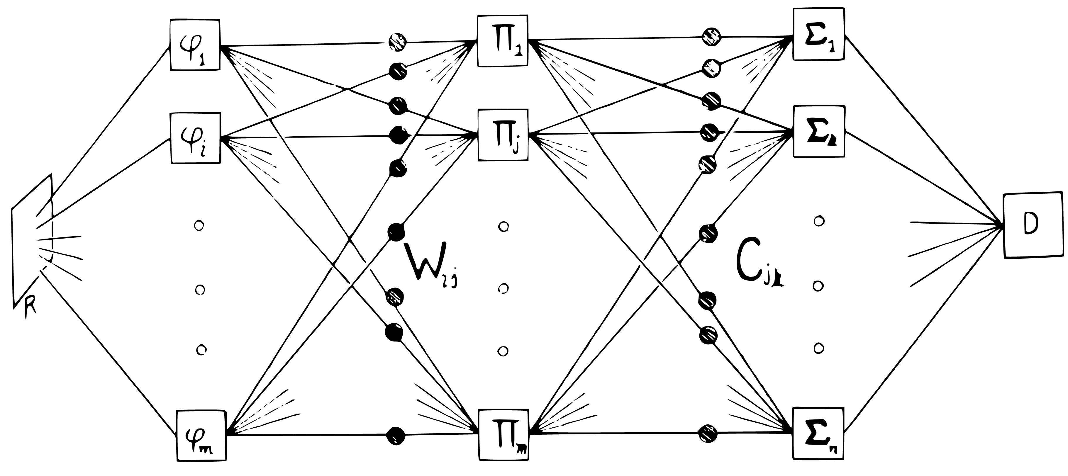
FIGURE 10.6: Layered perceptrons, as illustrated in the book Perceptrons
Before we start, let’s first install all the packages that we are about to use:
Using Spark we can create a multilayer perceptron classifier with ml_multilayer_perceptron_classifier() and gradient descent to classify and predict over large datasets. Gradient descent was introduced to layered perceptrons by Geoff Hinton.25
library(sparktf)
library(sparklyr)

sc <- spark_connect(master = "local", version = "2.3")

attrition <- copy_to(sc, rsample::attrition)

nn_model <- ml_multilayer_perceptron_classifier(
  attrition,
  Attrition ~ Age + DailyRate + DistanceFromHome + MonthlyIncome,
  layers = c(4, 3, 2),
  solver = "gd")

nn_model %>%
  ml_predict(attrition) %>%
  select(Attrition, predicted_label, starts_with("probability_")) %>%
  glimpse()
Observations: ??
Variables: 4
Database: spark_connection
$ Attrition <chr> "Yes", "No", "Yes", "No", "No", "No", "No", "No", "No"…
$ predicted_label <chr> "No", "No", "No", "No", "No", "No", "No", "No", "No", …
$ probability_No <dbl> 0.8439275, 0.8439275, 0.8439275, 0.8439275, 0.8439275,…
$ probability_Yes <dbl> 0.1560725, 0.1560725, 0.1560725, 0.1560725, 0.1560725,…Notice that the columns must be numeric, so you will need to manually convert them with the feature transforming techniques presented in Chapter 4. It is natural to try to add more layers to classify more complex datasets; however, adding too many layers will cause the gradient to vanish, and other techniques will need to use these deep layered networks, also known as deep learning models.
Deep learning models solve the vanishing gradient problem by making use of special activation functions, dropout, data augmentation and GPUs. You can use Spark to retrieve and preprocess large datasets into numerical-only datasets that can fit in a GPU for deep learning training. TensorFlow is one of the most popular deep learning frameworks. As mentioned previously, it supports a binary format known as TensorFlow records.
You can write TensorFlow records using the sparktf in Spark, which you can prepare to process in GPU instances with libraries like Keras or TensorFlow.
You can then preprocess large datasets in Spark and write them as TensorFlow records using spark_write_tf():
copy_to(sc, iris) %>%
  ft_string_indexer_model(
    "Species", "label",
    labels = c("setosa", "versicolor", "virginica")
  ) %>%
  spark_write_tfrecord(path = "tfrecord")
After you have trained the dataset with Keras or TensorFlow, you can use the tfdatasets package to load it. You will also need to install the TensorFlow runtime by using install_tensorflow() and install Python on your own. To learn more about training deep learning models with Keras, we recommend reading Deep Learning with R.26
<DatasetV1Adapter shapes: (), types: tf.string>Training deep learning models in a single local node with one or more GPUs is often enough for most applications; however, recent state-of-the-art deep learning models train using distributed computing frameworks like Apache Spark. Distributed computing frameworks are used to achieve higher petaflops each day the systems spends training these models. OpenAI analyzed trends in the field of artificial intelligence (AI) and cluster computing (illustrated in Figure 10.7). It should be obvious from the figure that there is a trend in recent years to use distributed computing frameworks.
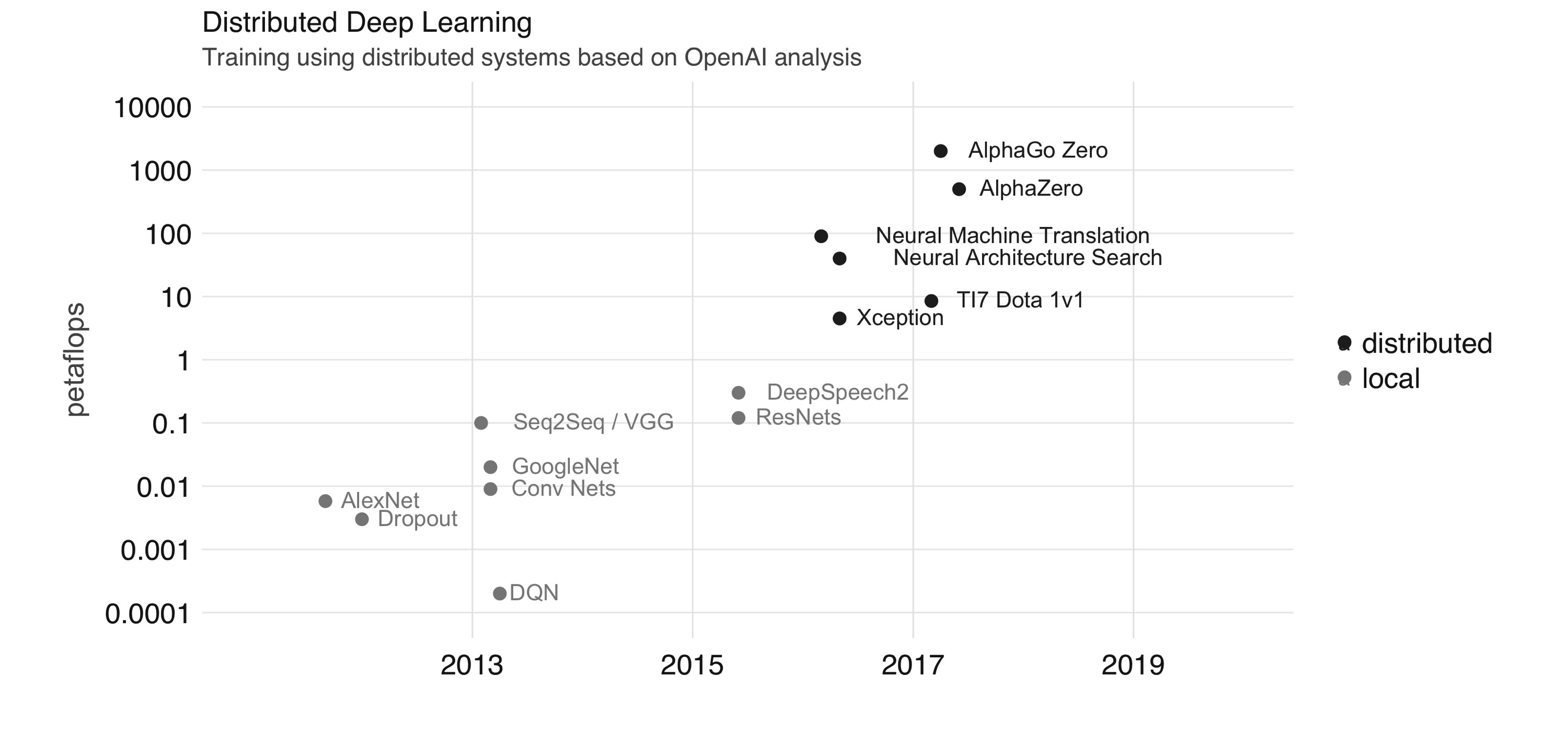
FIGURE 10.7: Training using distributed systems based on OpenAI analysis
Training large-scale deep learning models is possible in Spark and TensorFlow through frameworks like Horovod. Today, it’s possible to use Horovod with Spark from R using the reticulate package, since Horovod requires Python and Open MPI, this goes beyond the scope of this book. Next, we will introduce a different Spark extension in the domain of genomics.
10.6 Genomics
The human genome consists of two copies of about 3 billion base pairs of DNA within the 23 chromosome pairs. Figure 10.8 shows the organization of the genome into chromosomes. DNA strands are composed of nucleotides, each composed of one of four nitrogen-containing nucleobases: cytosine (C), guanine (G), adenine (A), or thymine (T). Since the DNA of all humans is nearly identical, we need to store only the differences from the reference genome in the form of a variant call format (VCF) file.
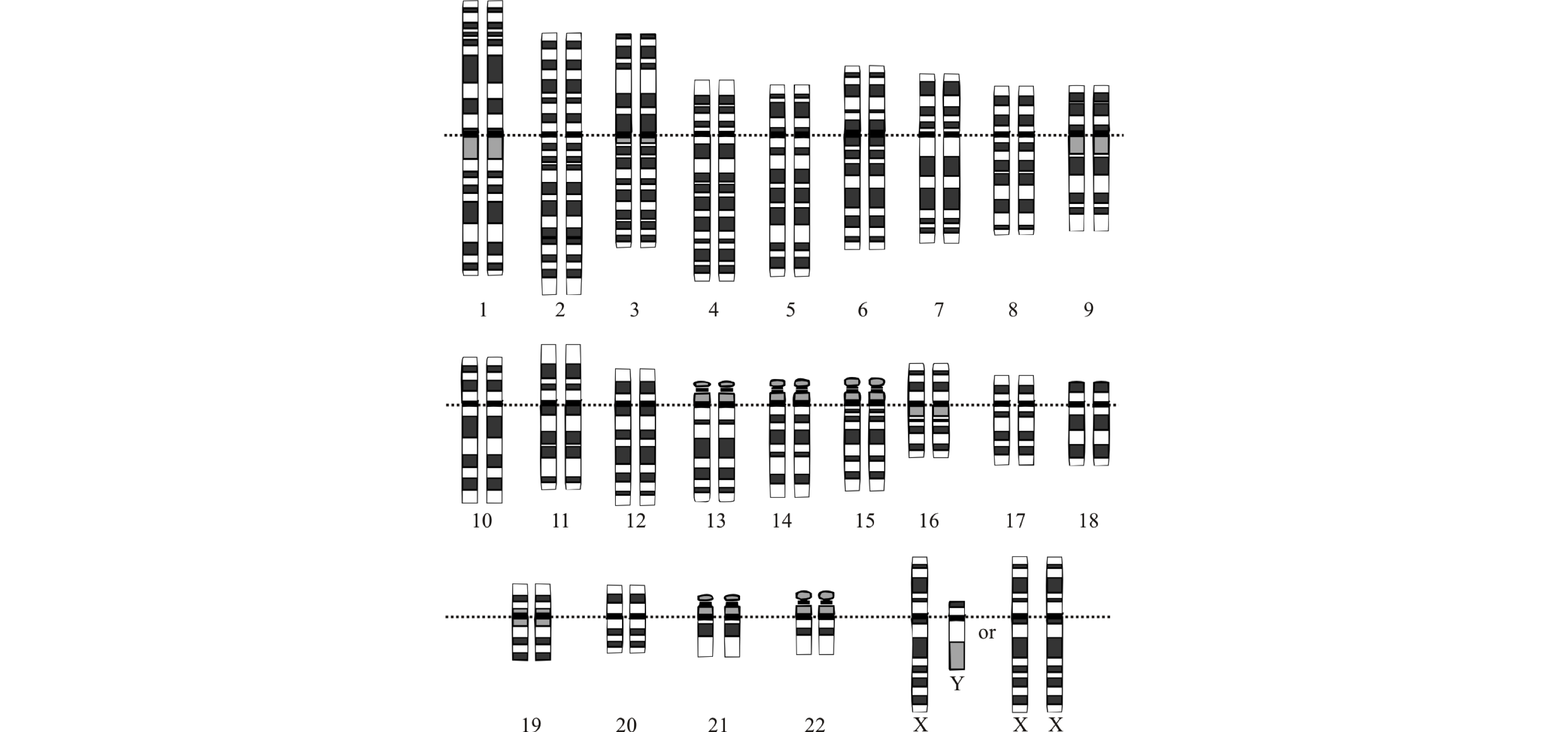
FIGURE 10.8: The idealized human diploid karyotype showing the organization of the genome into chromosomes
variantspark is a framework based on Scala and Spark to analyze genome datasets. It is being developed by CSIRO Bioinformatics team in Australia. variantspark was tested on datasets with 3,000 samples, each one containing 80 million features in either unsupervised clustering approaches or supervised applications, like classification and regression. variantspark can read VCF files and run analyses while using familiar Spark DataFrames.
To get started, install variantspark from CRAN, connect to Spark, and retrieve a vsc connection to variantspark:
library(variantspark)
library(sparklyr)

sc <- spark_connect(master = "local", version = "2.3",
                    config = list(sparklyr.connect.timeout = 3 * 60))

vsc <- vs_connect(sc)
We can start by loading a VCF file:
vsc_data <- system.file("extdata/", package = "variantspark")

hipster_vcf <- vs_read_vcf(vsc, file.path(vsc_data, "hipster.vcf.bz2"))
hipster_labels <- vs_read_csv(vsc, file.path(vsc_data, "hipster_labels.txt"))
labels <- vs_read_labels(vsc, file.path(vsc_data, "hipster_labels.txt"))
variantspark uses random forest to assign an importance score to each tested variant reflecting its association to the interest phenotype. A variant with higher importance score implies it is more strongly associated with the phenotype of interest. You can compute the importance and transform it into a Spark table, as follows:
importance_tbl <- vs_importance_analysis(vsc, hipster_vcf,
                                         labels, n_trees = 100) %>%
  importance_tbl()

importance_tbl
# Source: spark<?> [?? x 2]
variable importance
<chr> <dbl>
1 2_109511398 0
2 2_109511454 0
3 2_109511463 0.00000164
4 2_109511467 0.00000309
5 2_109511478 0
6 2_109511497 0
7 2_109511525 0
8 2_109511527 0
9 2_109511532 0
10 2_109511579 0
# … with more rowsYou then can use dplyr and ggplot2 to transform the output and visualize it (see Figure 10.9):
library(dplyr)
library(ggplot2)

importance_df <- importance_tbl %>%
  arrange(-importance) %>%
  head(20) %>%
  collect()

ggplot(importance_df) +
  aes(x = variable, y = importance) +
  geom_bar(stat = 'identity') +
  scale_x_discrete(limits =
    importance_df[order(importance_df$importance), 1]$variable) +
  coord_flip()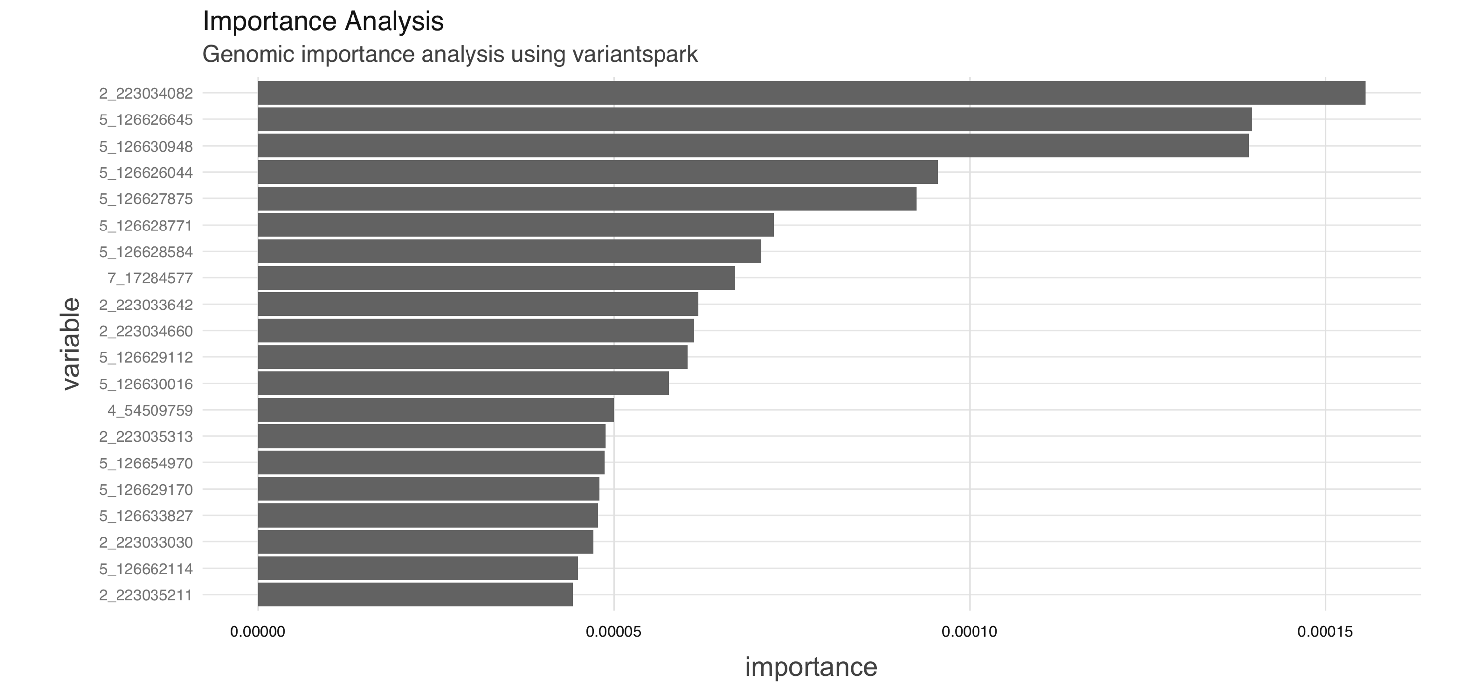
FIGURE 10.9: Genomic importance analysis using variantspark
This concludes a brief introduction to genomic analysis in Spark using the variantspark extension. Next, we move away from microscopic genes to macroscopic datasets that contain geographic locations across the world.
10.7 Spatial
geospark enables distributed geospatial computing using a grammar compatible with dplyr and sf, which provides a set of tools for working with geospatial vectors.
You can install geospark from CRAN, as follows:
Then, initialize the geospark extension and connect to Spark:
Next, we load a spatial dataset containing polygons and points:
polygons <- system.file("examples/polygons.txt", package="geospark") %>%
  read.table(sep="|", col.names = c("area", "geom"))

points <- system.file("examples/points.txt", package="geospark") %>%
  read.table(sep = "|", col.names = c("city", "state", "geom"))

polygons_wkt <- copy_to(sc, polygons)
points_wkt <- copy_to(sc, points)
There are various spatial operations defined in geospark, as depicted in Figure 10.10. These operations allow you to control how geospatial data should be queried based on overlap, intersection, disjoint sets, and so on.
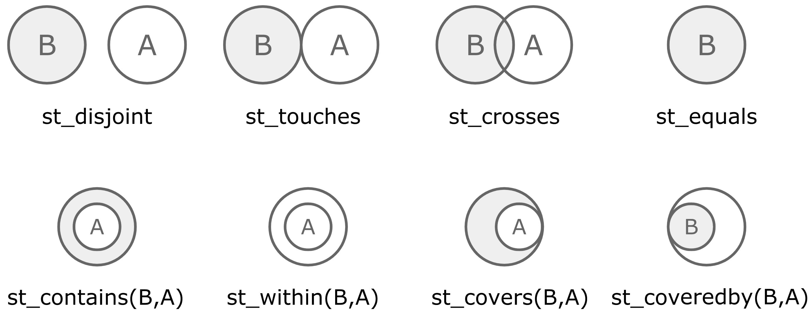
FIGURE 10.10: Spatial operations available in geospark
For instance, we can use these operations to find the polygons that contain a given set of points using st_contains():
library(dplyr)
polygons_wkt <- mutate(polygons_wkt, y = st_geomfromwkt(geom))
points_wkt <- mutate(points_wkt, x = st_geomfromwkt(geom))

inner_join(polygons_wkt,
           points_wkt,
           sql_on = sql("st_contains(y,x)")) %>%
  group_by(area, state) %>%
  summarise(cnt = n())
# Source: spark<?> [?? x 3]
# Groups: area
area state cnt
<chr> <chr> <dbl>
1 california area CA 10
2 new york area NY 9
3 dakota area ND 10
4 texas area TX 10
5 dakota area SD 1You can also plot these datasets by collecting a subset of the entire dataset or aggregating the geometries in Spark before collecting them. One package you should look into is sf.
We close this chapter by presenting a couple of troubleshooting techniques applicable to all extensions.
10.8 Troubleshooting
When you are using a new extension for the first time, we recommend increasing the connection timeout (given that Spark will usually need to download extension dependencies) and changing logging to verbose to help you troubleshoot when the download process does not complete:
config <- spark_config()
config$sparklyr.connect.timeout <- 3 * 60
config$sparklyr.log.console = TRUE

sc <- spark_connect(master = "local", config = config)
In addition, you should know that Apache IVY is a popular dependency manager focusing on flexibility and simplicity, and is used by Apache Spark for installing extensions. When the connection fails while you are using an extension, consider clearing your IVY cache by running the following:
In addition, you can also consider opening GitHub issues from the following extensions repositories to get help from the extension authors:
- rsparkling: github.com/h2oai/sparkling-water.
- sparkxgb: github.com/rstudio/sparkxgb.
- sparktf: github.com/rstudio/sparktf.
- variantspark: github.com/r-spark/variantspark.
- geospark: github.com/r-spark/geospark.
10.9 Recap
This chapter provided a brief overview on using some of the Spark extensions available in R, which happens to be as easy as installing a package. You then learned how to use the rsparkling extension, which provides access to H2O in Spark, which in turn provides additional modeling functionality like enhanced metrics and the ability to automatically select models. We then jumped to graphframes, an extension to help you process relational datasets that are formally referred to as graphs. You also learned how to compute simple connection metrics or run complex algorithms like PageRank.
The XGBoost and deep learning sections provided alternate modeling techniques that use gradient descent: the former over decision trees, and the latter over deep multilayered perceptrons where we can use Spark to preprocess datasets into records that later can be consumed by TensorFlow and Keras using the sparktf extension. The last two sections introduced extensions to process genomic and spatial datasets through the variantspark and geospark extensions.
These extensions, and many more, provide a comprehensive library of advanced functionality that, in combination with the analysis and modeling techniques presented, should cover most tasks required to run in computing clusters. However, when functionality is lacking, you can consider writing your own extension, which is what we discuss in Chapter 13, or you can apply custom transformations over each partition using R code, as we describe in Chapter 11.
Notice that AutoML uses cross-validation, which we did not use in GLM.↩
Rosenblatt F (1958). “The perceptron: a probabilistic model for information storage and organization in the brain.” Psychological review.↩
Minsky M, Papert SA (2017). Perceptrons: An introduction to computational geometry. MIT press.↩
Ackley DH, Hinton GE, Sejnowski TJ (1985). “A learning algorithm for Boltzmann machines.” Cognitive science.↩
Chollet F, Allaire J (2018). Deep Learning with R. Manning Publications.↩