Chapter 1 Introduction

You know nothing, Jon Snow.

— Ygritte

With information growing at exponential rates, it’s no surprise that historians are referring to this period of history as the Information Age. The increasing speed at which data is being collected has created new opportunities and is certainly poised to create even more. This chapter presents the tools that have been used to solve large-scale data challenges. First, it introduces Apache Spark as a leading tool that is democratizing our ability to process large datasets. With this as a backdrop, we introduce the R computing language, which was specifically designed to simplify data analysis. Finally, this leads us to introduce sparklyr, a project merging R and Spark into a powerful tool that is easily accessible to all.

Chapter 2 presents the prerequisites, tools, and steps you need to perform to get Spark and R working on your personal computer. You will learn how to install and initialize Spark, get introduced to common operations, and get your very first data processing and modeling task done. It is the goal of that chapter to help anyone grasp the concepts and tools required to start tackling large-scale data challenges which, until recently, were accessible to just a few organizations.

You then move into learning how to analyze large-scale data, followed by building models capable of predicting trends and discover information hidden in vast amounts of information. At which point, you will have the tools required to perform data analysis and modeling at scale. Subsequent chapters help you move away from your local computer into computing clusters required to solve many real world problems. The last chapters present additional topics, like real-time data processing and graph analysis, which you will need to truly master the art of analyzing data at any scale. The last chapter of this book provides you with tools and inspiration to consider contributing back to the Spark and R communities.

We hope that this is a journey you will enjoy, that will help you to solve problems in your professional career, and to nudge the world into making better decisions that can benefit us all.

1.1 Overview

As humans, we have been storing, retrieving, manipulating, and communicating information since the Sumerians in Mesopotamia developed writing around 3000 BC. Based on the storage and processing technologies employed, it is possible to distinguish four distinct phases of development: premechanical (3000 BC to 1450 AD), mechanical (1450–1840), electromechanical (1840–1940), and electronic (1940–present).¹

Mathematician George Stibitz used the word digital to describe fast electric pulses back in 1942,² and to this day, we describe information stored electronically as digital information. In contrast, analog information represents everything we have stored by any nonelectronic means such as handwritten notes, books, newspapers, and so on.

The World Bank report on digital development provides an estimate of digital and analog information stored over the past decades.³ This report noted that digital information surpassed analog information around 2003. At that time, there were about 10 million terabytes of digital information, which is roughly about 10 million storage drives today. However, a more relevant finding from this report was that our footprint of digital information is growing at exponential rates. Figure 1.1 shows the findings of this report; notice that every other year, the world’s information has grown tenfold.

FIGURE 1.1: World’s capacity to store information

With the ambition to provide tools capable of searching all of this new digital information, many companies attempted to provide such functionality with what we know today as search engines, used when searching the web. Given the vast amount of digital information, managing information at this scale was a challenging problem. Search engines were unable to store all of the web page information required to support web searches in a single computer. This meant that they had to split information into several files and store them across many machines. This approach became known as the Google File System, and was presented in a research paper published in 2003 by Google.⁴

1.2 Hadoop

One year later, Google published a new paper describing how to perform operations across the Google File System, an approach that came to be known as MapReduce.⁵ As you would expect, there are two operations in MapReduce: map and reduce. The map operation provides an arbitrary way to transform each file into a new file, whereas the reduce operation combines two files. Both operations require custom computer code, but the MapReduce framework takes care of automatically executing them across many computers at once. These two operations are sufficient to process all the data available on the web, while also providing enough flexibility to extract meaningful information from it.

For example, as illustrated in Figure 1.2, we can use MapReduce to count words in two different text files stored in different machines. The map operation splits each word in the original file and outputs a new word-counting file with a mapping of words and counts. The reduce operation can be defined to take two word-counting files and combine them by aggregating the totals for each word; this last file will contain a list of word counts across all the original files.

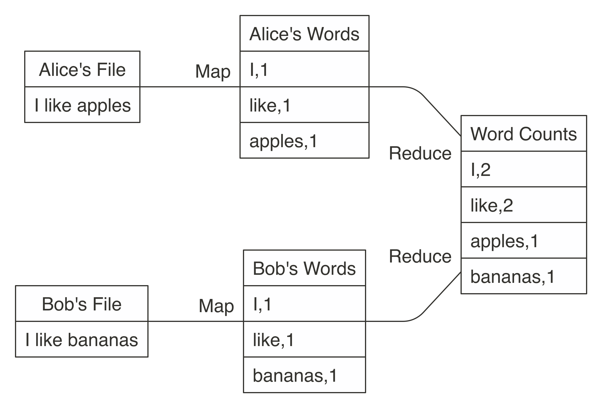
FIGURE 1.2: MapReduce example counting words across files

Counting words is often the most basic MapReduce example, but we can also use MapReduce for much more sophisticated and interesting applications. For instance, we can use it to rank web pages in Google’s PageRank algorithm, which assigns ranks to web pages based on the count of hyperlinks linking to a web page and the rank of the page linking to it.

After these papers were released by Google, a team at Yahoo worked on implementing the Google File System and MapReduce as a single open source project. This project was released in 2006 as Hadoop, with the Google File System implemented as the Hadoop Distributed File System (HDFS). The Hadoop project made distributed file-based computing accessible to a wider range of users and organizations, making MapReduce useful beyond web data processing.

Although Hadoop provided support to perform MapReduce operations over a distributed file system, it still required MapReduce operations to be written with code every time a data analysis was run. To improve upon this tedious process, the Hive project, released in 2008 by Facebook, brought Structured Query Language (SQL) support to Hadoop. This meant that data analysis could now be performed at large scale without the need to write code for each MapReduce operation; instead, one could write generic data analysis statements in SQL, which are much easier to understand and write.

1.3 Spark

In 2009, Apache Spark began as a research project at UC Berkeley’s AMPLab to improve on MapReduce. Specifically, Spark provided a richer set of verbs beyond MapReduce to facilitate optimizing code running in multiple machines. Spark also loaded data in-memory, making operations much faster than Hadoop’s on-disk storage. One of the earliest results showed that running logistic regression, a data modeling technique that we will introduce in Chapter 4, allowed Spark to run 10 times faster than Hadoop by making use of in-memory datasets.⁶. A chart similar to Figure 1.3 was presented in the original research publication.

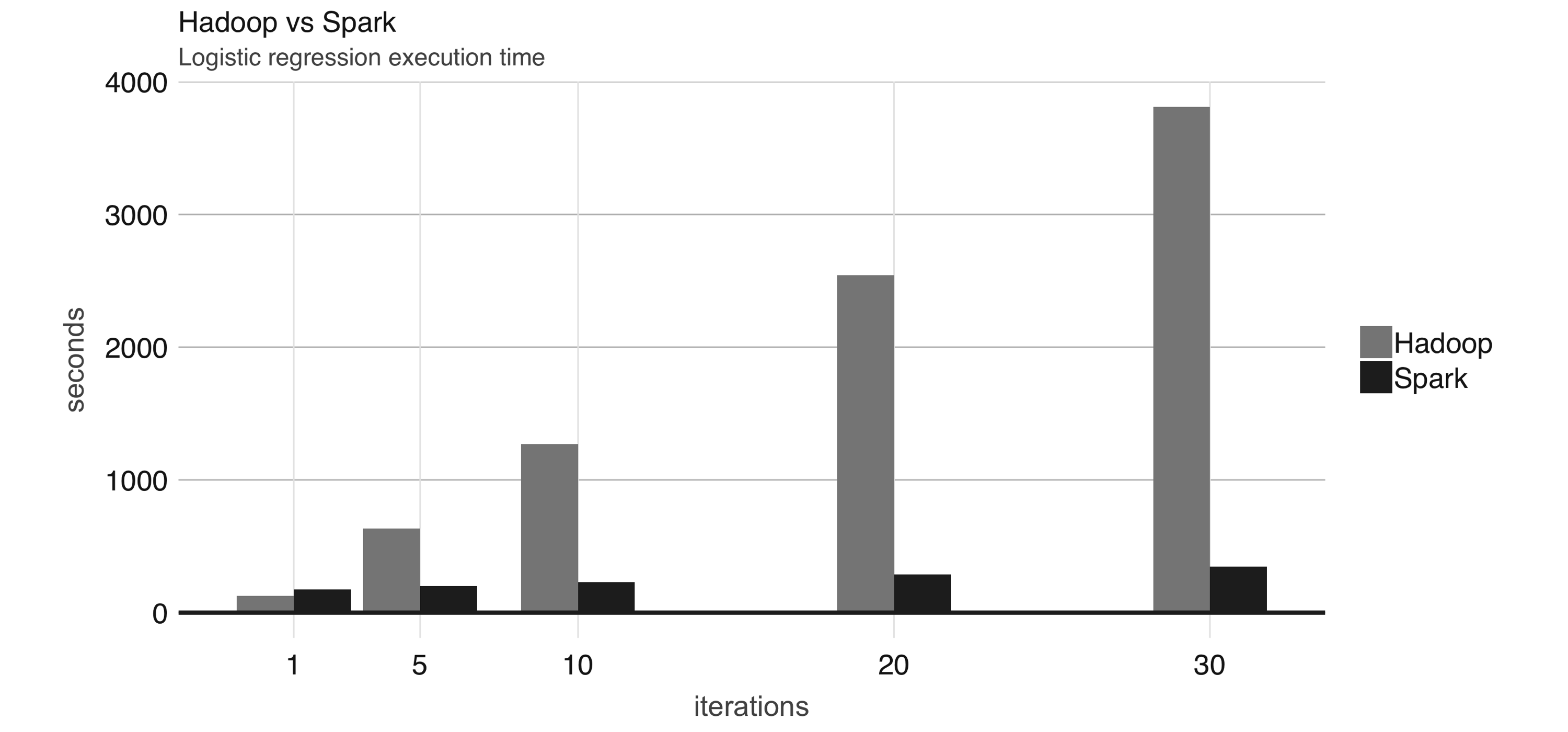
FIGURE 1.3: Logistic regression performance in Hadoop and Spark

Even though Spark is well known for its in-memory performance, it was designed to be a general execution engine that works both in-memory and on-disk. For instance, Spark has set sorting⁷, for which data was not loaded in-memory; rather, Spark made improvements in network serialization, network shuffling, and efficient use of the CPU’s cache to dramatically enhance performance. If you needed to sort large amounts of data, there was no other system in the world faster than Spark.

To give you a sense of how much faster and efficient Spark is, it takes 72 minutes and 2,100 computers to sort 100 terabytes of data using Hadoop, but only 23 minutes and 206 computers using Spark. In addition, Spark holds the cloud sorting record, which makes it the most cost-effective solution for sorting large-datasets in the cloud.

	Hadoop Record	Spark Record
Data Size	102.5 TB	100 TB
Elapsed Time	72 mins	23 mins
Nodes	2100	206
Cores	50400	6592
Disk	3150 GB/s	618 GB/s
Network	10Gbps	10Gbps
Sort rate	1.42 TB/min	4.27 TB/min
Sort rate / node	0.67 GB/min	20.7 GB/min

Spark is also easier to use than Hadoop; for instance, the word-counting MapReduce example takes about 50 lines of code in Hadoop, but it takes only 2 lines of code in Spark. As you can see, Spark is much faster, more efficient, and easier to use than Hadoop.

In 2010, Spark was released as an open source project and then donated to the Apache Software Foundation in 2013. Spark is licensed under Apache 2.0, which allows you to freely use, modify, and distribute it. Spark then reached more than 1,000 contributors, making it one of the most active projects in the Apache Software Foundation.

This gives an overview of how Spark came to be, which we can now use to formally introduce Apache Spark as defined on the project’s website:

Apache Spark is a unified analytics engine for large-scale data processing.

— spark.apache.org

To help us understand this definition of Apache Spark, we break it down as follows:

Unified: Spark supports many libraries, cluster technologies, and storage systems.
Analytics: Analytics is the discovery and interpretation of data to produce and communicate information.
Engine: Spark is expected to be efficient and generic.
Large-Scale: You can interpret large-scale as cluster-scale, a set of connected computers working together.

Spark is described as an engine because it’s generic and efficient. It’s generic because it optimizes and executes generic code; that is, there are no restrictions as to what type of code you can write in Spark. It is efficient, because, as we mentioned earlier, Spark much faster than other technologies by making efficient use of memory, network, and CPUs to speed data processing algorithms in computing clusters.

This makes Spark ideal in many analytics projects like ranking movies at Netflix, aligning protein sequences, or analyzing high-energy physics at CERN.

As a unified platform, Spark is expected to support many cluster technologies and multiple data sources, which you learn about in Chapter 6 and Chapter 8, respectively. It is also expected to support many different libraries like Spark SQL, MLlib, GraphX, and Spark Streaming; libraries that you can use for analysis, modeling, graph processing, and real-time data processing, respectively. In summary, Spark is a platform providing access to clusters, data sources, and libraries for large-scale computing, as illustrated in Figure 1.4.

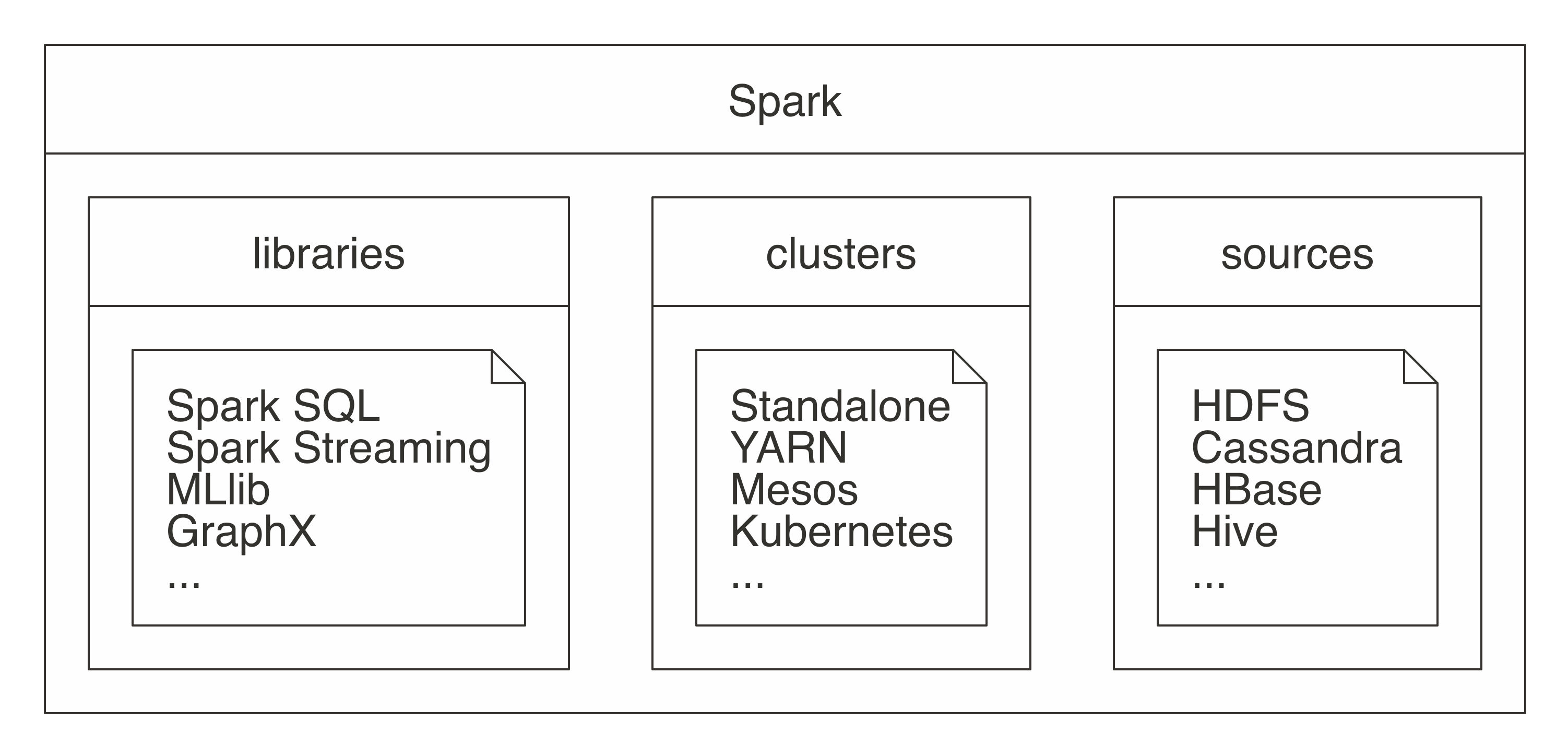
FIGURE 1.4: Spark as a unified analytics engine for large-scale data processing

Describing Spark as large scale implies that a good use case for Spark is tackling problems that can be solved with multiple machines. For instance, when data does not fit on a single disk drive or into memory, Spark is a good candidate to consider. However, you can also consider it for problems that might not be large scale, but for which using multiple computers could speed up computation. For instance, CPU-intensive models and scientific simulations also benefit from running in Spark.

Therefore, Spark is good at tackling large-scale data-processing problems, usually known as big data (datasets that are more voluminous and complex than traditional ones) but it is also good at tackling large-scale computation problems, known as big compute (tools and approaches using a large amount of CPU and memory resources in a coordinated way). Big data often requires big compute, but big compute does not necessarily require big data.

Big data and big compute problems are usually easy to spot—if the data does not fit into a single machine, you might have a big data problem; if the data fits into a single machine but processing it takes days, weeks, or even months to compute, you might have a big compute problem.

However, there is also a third problem space for which neither data nor compute is necessarily large scale and yet there are significant benefits to using cluster computing frameworks like Spark. For this third problem space, there are a few use cases:

Velocity: Suppose that you have a dataset of 10 GB and a process that takes 30 minutes to run over this data—this is neither big compute nor big data by any means. However, if you happen to be researching ways to improve the accuracy of your models, reducing the runtime down to three minutes is a significant improvement, which can lead to meaningful advances and productivity gains by increasing the velocity at which you can analyze data. Alternatively, you might need to process data faster—for stock trading, for instance. Whereas three minutes could seem fast enough, it can be far too slow for real-time data processing, for which you might need to process data in a few seconds—or even a few milliseconds.
Variety: You could also have an efficient process to collect data from many sources into a single location, usually a database; this process could be already running efficiently and close to real time. Such processes are known as Extract, Transform, Load (ETL); data is extracted from multiple sources, transformed to the required format, and loaded into a single data store. Although this has worked for years, the trade-off from this approach is that adding a new data source is expensive. Because the system is centralized and tightly controlled, making changes could cause the entire process to halt; therefore, adding new data source usually takes too long to be implemented. Instead, you can store all data in its natural format and process it as needed using cluster computing, an architecture known as a data lake. In addition, storing data in its raw format allows you to process a variety of new file formats like images, audio, and video without having to figure out how to fit them into conventional structured storage systems.
Veracity: When using many data sources, you might find the data quality varies greatly between them, which requires special analysis methods to improve their accuracy. For instance, suppose that you have a table of cities with values like San Francisco, Seattle, and Boston. What happens when data contains a misspelled entry like “Bston”? In a relational database, this invalid entry might be dropped. However, dropping values is not necessarily the best approach in all cases; you might want to correct this field by making use of geocodes, cross-referencing data sources, or attempting a best-effort match. Therefore, understanding and improving the veracity of the original data source can lead to more accurate results.

If we include “volume” as a synonym for big data, you get the mnemonic people refer to as the four Vs of big data; others have expanded this to five or even 10 Vs of big data. Mnemonics aside, cluster computing is being used today in more innovative ways, and is not uncommon to see organizations experimenting with new workflows and a variety of tasks that were traditionally uncommon for cluster computing. Much of the hype attributed to big data falls into this space where, strictly speaking, you’re not handling big data, but there are still benefits from using tools designed for big data and big compute.

Our hope is that this book will help you to understand the opportunities and limitations of cluster computing and, specifically, the opportunities and limitations of using Apache Spark with R.

1.4 R

The R computing language has its origins in the S language, which was created at Bell Laboratories. Rick Becker explained in useR 2016 that at that time in Bell Labs, computing was done by calling subroutines written in the Fortran language, which, apparently, were not pleasant to deal with. The S computing language was designed as an interface language to solve particular problems without having to worry about other languages, such as Fortran. The creator of S, John Chambers, shows in Figure 1.5 how S was designed to provide an interface that simplifies data processing; his co-creator presented this during useR! 2016 as the original diagram that inspired the creation of S.

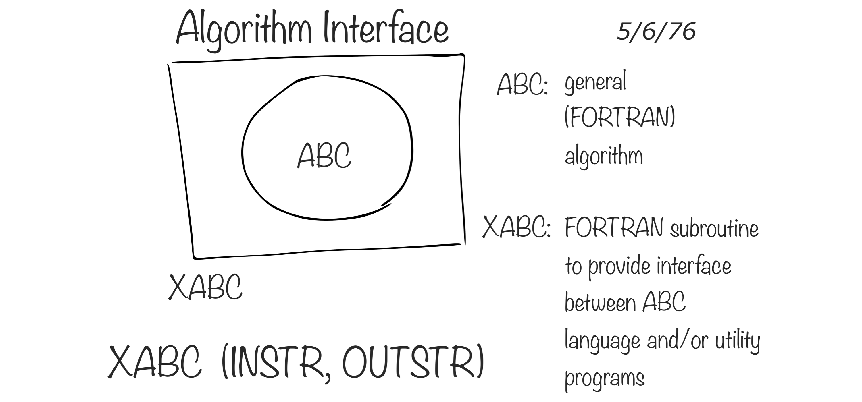
FIGURE 1.5: Interface language diagram by John Chambers (Rick Becker useR 2016)

R is a modern and free implementation of S. Specifically, according to the R Project for Statistical Computing:

R is a programming language and free software environment for statistical computing and graphics.

While working with data, we believe there are two strong arguments for using R:

R Language: R was designed by statisticians for statisticians, meaning that this is one of the few successful languages designed for nonprogrammers, so learning R will probably feel more natural. Additionally, because the R language was designed to be an interface to other tools and languages, R allows you to focus more on understanding data and less on the particulars of computer science and engineering.
R Community: The R community provides a rich package archive provided by the Comprehensive R Archive Network (CRAN), which allows you to install ready-to-use packages to perform many tasks—most notably high-quality data manipulation, visualization, and statistical models, many of which are available only in R. In addition, the R community is a welcoming and active group of talented individuals motivated to help you succeed. Many packages provided by the R community make R, by far, the best option for statistical computing. Some of the most downloaded R packages include: dplyr to manipulate data, cluster to analyze clusters, and ggplot2 to visualize data. Figure 1.6 quantifies the growth of the R community by plotting daily downloads of R packages in CRAN.

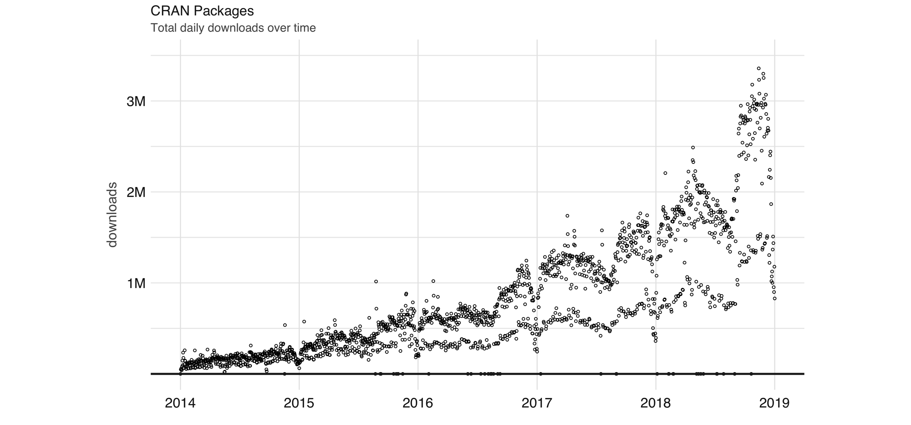
FIGURE 1.6: Daily downloads of CRAN packages

Aside from statistics, R is also used in many other fields. The following areas are particularly relevant to this book:

Data Science: Data science is based on knowledge and practices from statistics and computer science that turn raw data into understanding⁸ by using data analysis and modeling techniques. Statistical methods provide a solid foundation to understand the world and perform predictions, while the automation provided by computing methods allows us to simplify statistical analysis and make it much more accessible. Some have advocated that statistics should be renamed data science;⁹ however, data science goes beyond statistics by also incorporating advances in computing.¹⁰ This book presents analysis and modeling techniques common in statistics but applied to large datasets, which requires incorporating advances in distributed computing.
Machine Learning: Machine learning uses practices from statistics and computer science; however, it is heavily focused on automation and prediction. For instance, Arthur Samuel coined the term machine learning while automating a computer program to play checkers.¹¹ Although we could perform data science on particular games, writing a program to play checkers requires us to automate the entire process. Therefore, this falls in the realm of machine learning, not data science. Machine learning makes it possible for many users to take advantage of statistical methods without being aware of using them. One of the first important applications of machine learning was to filter spam emails. In this case, it’s just not feasible to perform data analysis and modeling over each email account; therefore, machine learning automates the entire process of finding spam and filtering it out without having to involve users at all. This book presents the methods to transition data science workflows into fully automated machine learning methods—for instance, by providing support to build and export Spark pipelines that can be easily reused in automated environments.
Deep Learning: Deep learning builds on knowledge of statistics, data science, and machine learning to define models loosely inspired by biological nervous systems. Deep learning models evolved from neural network models after the vanishing-gradient problem was resolved by training one layer at a time,¹² and have proven useful in image and speech recognition tasks. For instance, in voice assistants like Siri, Alexa, Cortana, or Google Assistant, the model performing the audio-to-text conversion is most likely based on deep learning models. Although Graphic Processing Units (GPUs) have been successfully used to train deep learning models,¹³ some datasets cannot be processed in a single GPU. It is also the case that deep learning models require huge amounts of data, which needs to be preprocessed across many machines before it can be fed into a single GPU for training. This book doesn’t make any direct references to deep learning models; however, you can use the methods we present in this book to prepare data for deep learning and, in the years to come, using deep learning with large-scale computing will become a common practice. In fact, recent versions of Spark have already introduced execution models optimized for training deep learning in Spark.

When working in any of the previous fields, you will be faced with increasingly large datasets or increasingly complex computations that are slow to execute or at times even impossible to process in a single computer. However, it is important to understand that Spark does not need to be the answer to all our computations problems; instead, when faced with computing challenges in R, using the following techniques can be as effective:

Sampling: A first approach to try is to reduce the amount of data being handled, through sampling. However, we must sample the data properly by applying sound statistical principles. For instance, selecting the top results is not sufficient in sorted datasets; with simple random sampling, there might be underrepresented groups, which we could overcome with stratified sampling, which in turn adds complexity to properly select categories. It’s beyond the scope of this book to teach how to properly perform statistical sampling, but many resources are available on this topic.
Profiling: You can try to understand why a computation is slow and make the necessary improvements. A profiler is a tool capable of inspecting code execution to help identify bottlenecks. In R, the R profiler, the profvis R package, and RStudio profiler feature allow you to easily to retrieve and visualize a profile; however, it’s not always trivial to optimize.
Scaling Up: Speeding up computation is usually possible by buying faster or more capable hardware (say, increasing your machine memory, upgrading your hard drive, or procuring a machine with many more CPUs); this approach is known as scaling up. However, there are usually hard limits as to how much a single computer can scale up, and even with significant CPUs, you need to find frameworks that parallelize computation efficiently.
Scaling Out: Finally, we can consider spreading computation and storage across multiple machines. This approach provides the highest degree of scalability because you can potentially use an arbitrary number of machines to perform a computation. This approach is commonly known as scaling out. However, spreading computation effectively across many machines is a complex endeavor, especially without using specialized tools and frameworks like Apache Spark.

This last point brings us closer to the purpose of this book, which is to bring the power of distributed computing systems provided by Apache Spark to solve meaningful computation problems in data science and related fields, using R.

1.5 sparklyr

When you think of the computation power that Spark provides and the ease of use of the R language, it is natural to want them to work together, seamlessly. This is also what the R community expected: an R package that would provide an interface to Spark that was easy to use, compatible with other R packages, and available in CRAN. With this goal, we started developing sparklyr. The first version, sparklyr 0.4, was released during the useR! 2016 conference. This first version included support for dplyr, DBI, modeling with MLlib, and an extensible API that enabled extensions like H2O’s rsparkling package. Since then, many new features and improvements have been made available through sparklyr 0.5, 0.6, 0.7, 0.8, 0.9 and 1.0.

Officially, sparklyr is an R interface for Apache Spark. It’s available in CRAN and works like any other CRAN package, meaning that it’s agnostic to Spark versions, it’s easy to install, it serves the R community, it embraces other packages and practices from the R community, and so on. It’s hosted in GitHub and licensed under Apache 2.0, which allows you to clone, modify, and contribute back to this project.

When thinking of who should use sparklyr, the following roles come to mind:

New Users: For new users, it is our belief that sparklyr provides the easiest way to get started with Spark. Our hope is that the early chapters of this book will get you up and running with ease and set you up for long-term success.
Data Scientists: For data scientists who already use and love R, sparklyr integrates with many other R practices and packages like dplyr, magrittr, broom, DBI, tibble, rlang, and many others, which will make you feel at home while working with Spark. For those new to R and Spark, the combination of high-level workflows available in sparklyr and low-level extensibility mechanisms make it a productive environment to match the needs and skills of every data scientist.
Expert Users: For those users who are already immersed in Spark and can write code natively in Scala, consider making your Spark libraries available as an R package to the R community, a diverse and skilled community that can put your contributions to good use while moving open science forward.

We wrote this book to describe and teach the exciting overlap between Apache Spark and R. sparklyr is the R package that brings together these communities, expectations, future directions, packages, and package extensions. We believe that there is an opportunity to use this book to bridge the R and Spark communities: to present to the R community why Spark is exciting, and to the Spark community what makes R great. Both communities are solving very similar problems with a set of different skills and backgrounds; therefore, it is our hope that sparklyr can be a fertile ground for innovation, a welcoming place for newcomers, a productive environment for experienced data scientists, and an open community where cluster computing, data science, and machine learning can come together.

1.6 Recap

This chapter presented Spark as a modern and powerful computing platform, R as an easy-to-use computing language with solid foundations in statistical methods, and sparklyr as a project bridging both technologies and communities. In a world in which the total amount of information is growing exponentially, learning how to analyze data at scale will help you to tackle the problems and opportunities humanity is facing today. However, before we start analyzing data, Chapter 2 will equip you with the tools you will need throughout the rest of this book. Be sure to follow each step carefully and take the time to install the recommended tools, which we hope will become familiar resources that you use and love.

Laudon KC, Traver CG, Laudon JP (1996). “Information technology and systems.” Cambridge, MA: Course Technology.↩
Ceruzzi PE (2012). Computing: a concise history. MIT Press.↩
Group WB (2016). The Data Revolution. World Bank Publications.↩
Ghemawat S, Gobioff H, Leung S (2003). “The Google File System.” In Proceedings of the Nineteenth ACM Symposium on Operating Systems Principles. ISBN 1-58113-757-5.↩
Dean J, Ghemawat S (2004). “MapReduce: Simplified data processing on large clusters.” In USENIX Symposium on Operating System Design and Implementation (OSDI).↩
Zaharia M, Chowdhury M, Franklin MJ, Shenker S, Stoica I (2010). “Spark: Cluster computing with working sets.” HotCloud, 10(10-10), 95.↩
Zaharia M, Chowdhury M, Franklin MJ, Shenker S, Stoica I (2010). “Spark: Cluster computing with working sets.” HotCloud, 10(10-10), 95.↩
Wickham H, Grolemund G (2016). R for data science: import, tidy, transform, visualize, and model data. O’Reilly Media, Inc.↩
Wu CJ (1997). “Statistics = Data Science?”↩
Cleveland WS (2001). “Data Science: An Action Plan for Expanding the Technical Areas of the Field of Statistics?”↩
Samuel AL (1959). “Some studies in machine learning using the game of checkers.” IBM Journal of research and development, 3(3), 210–229.↩
Hinton GE, Osindero S, Teh Y (2006). “A fast learning algorithm for deep belief nets.” Neural computation, 18(7), 1527–1554.↩
Krizhevsky A, Sutskever I, Hinton GE (2012). “Imagenet classification with deep convolutional neural networks.” In Advances in neural information processing systems, 1097–1105.↩